Introduction
Few years ago I did some simple synthetic-aperture radar (SAR) imaging experiments with the second version of my homemade FMCW radar. Since then I made a much improved third version of the radar but didn't do any SAR measurements due to the amount of effort it would have required. I did have plans to do some SAR experiments afterwards but it took until now to have enough time and motivation.
Synthetic aperture radar (SAR) imaging is a way to synthesize very large antenna array by moving single antenna on a known path. If there are no moving targets in the scene then one radar taking many measurements along a path gives the same result as one ridiculously large radar that is as long as the movement path.
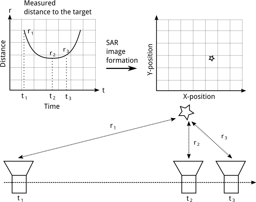
SAR imaging of a single target. As the radar moves the measured distance follows a parabola.
If we move on a straight path while radar pointing 90 degrees from the direction of the path measures a distance to the single target, we will find that the measured distance follows a parabola. This follows directly from the Pythagorean theorem. The SAR imaging problem is finding out the target position from the measured distance data. Of course in a real scene we have multiple targets and the solution isn't as simple as looking where the closest approach is as could be done in the picture above.
Omega-k algorithm
There are few different algorithms for solving this problem, but the one I'm going to use is called Omega-k algorithm. It is a fast imaging algorithm utilizing FFT which also makes it efficient to calculate on GPU. The derivation mostly follows a paper by Guo and Dong.
The radar I have is a frequency modulated constant wave (FMCW) radar. It transmits a short frequency sweep. The transmitted waveform can be modeled as:
, where \(j = \sqrt{-1}\), \(f_c =\) RF carrier frequency, \(\tau =\) time variable, \(\gamma = B/T_s =\) sweep bandwidth / sweep length \(=\) sweep rate.
The transmitted wave reflects off a target at some distance and is received after time \(t_d\). Ignoring the amplitude, the received wave is a time-delayed copy of the transmitted signal: \(s_r(\tau) = s_t(\tau - t_d)\). Signals from multiple targets are summed.
The receiver mixes the received signal with the transmitted signal. This mixing is called dechirping and it removes the high frequency RF component. The result is a low frequency signal, usually some few kHz to MHz and is easy to digitize with low-cost ADC. With the complex signals we take complex conjugate of the transmitted signal to get the low-pass product and the resulting mixing product is:
During SAR measurement the radar repeats this measurement while moving on a straight path with a constant speed. The position of the radar on the path is: \(x = v \tau + x_n\), where \(v\) is speed of the radar platform and \(x_n = v n T_p\). \(n\) is the index for measurements and \(T_p\) is the transmit repetition interval.
If the radar target is at position \((x_0, y_0)\) the distance to the target can be written as:
We set the y-coordinate of the path to be 0 and x position is limited to \(-L/2 < x < L/2\), where \(L\) is length of the path.
Since electromagnetic waves travel at the speed of light and radar signal needs to travel to the target and back to the radar, we get expression for received signal time delay \(t_d = 2R(x)/c\), where \(c\) is the speed of light.
The recorded signal can be written as:
The last term in the above expression is called residual video phase term and it's an undesirable by-product from dechirping operation. It should be removed before further processing by multiplying by \(\exp(-j \frac{4 \pi \gamma^2}{c^2} R^2(x))\). However this form is inconvenient because it depends on \(R(x)\). Using the fact that \(R(x) = c t_d / 2\) and that \(t_d\) can be expressed in terms of frequency of the IF signal: \(f = -2 \gamma R(x) / c = -\gamma t_d \Rightarrow t_d = -\frac{f}{\gamma}\) we can write the correction term as \(\exp(-j \pi f^2 / \gamma)\). This form can be applied easily to the Fourier transformed signal.
With RVP term removed the signal is:
Ideally we would like to have the signal in form \(\exp(-j 2 \pi f_y y_0)\exp(-j 2\pi f_x x_0)\), then we could apply two dimensional inverse Fourier transform to get a delta function centered at \((x_0, y_0)\) focusing the image. Currently the signal \(s(\tau, x_n)\) is not in this form and inverse Fourier transform doesn't give anything interesting. We need to find some processing steps to apply to the signal to get it to the required form so that inverse Fourier transform can be applied. The reason to look specifically for this kind of form is that FFT can be performed very efficiently.
As a first step, note that \(\gamma\) has units of Hz/s and \(\tau\) has units of s. The product \(\gamma \tau\) has units of Hz so it's a frequency. This product is actually instantenous modulation frequency of the sweep. We do substitution \(\gamma \tau \rightarrow f_\tau\) to get rid of the time variable. \(\tau\) range was \(-T/2 \ldots T/2\) and the new range for \(f_\tau\) is \(-B/2 \ldots B/2\).
Also instead of using frequency the math is cleaner and the implementation of the algorithm is easier when using wavenumbers instead. We define range wavenumber \(K_r = K_{rc} + \Delta K_r\). \(K_{rc} = \frac{4\pi f_c}{c}\), \(\Delta K_r = \frac{4\pi f_\tau}{c} = -\frac{2\pi B}{c} \ldots \frac{2\pi B}{c}\).
Next step is to do Fourier transform in azimuth direction (direction of the movement) to move also the \(x_n\) variable to frequency domain.
\(K_x = 2\pi f_x\) is wavenumber in the azimuth direction. This integral doesn't have exact solution, but there is a method to calculate quite accurate approximation using a method called principle of stationary phase (PSOP). Phase of the function being integrated can be written as:
If we plot the phase \(\Phi(x_n)\) for some realistic values we get a plot that looks something like below:
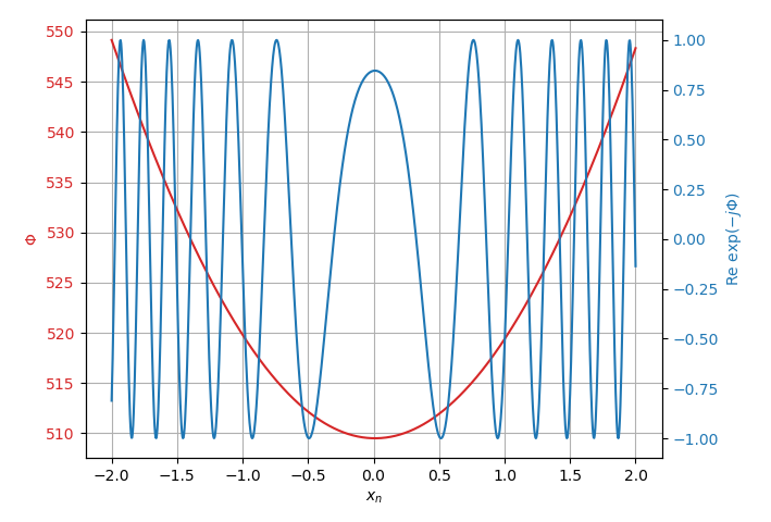
Phase and real part of the function being integrated.
There is one point where derivative of the phase is zero (stationary point) and the function varies slowly, but away from that point the function is highly oscillatory. As we integrate the function the oscillations far away from the stationary point cancel out and mainly the area around the stationary point contributes to the result of the integral.
We can expand the function around the stationary point \(\frac{d}{dx_n}\Phi(x_n) \rvert_{x_n=x_n^\star} = 0\), as \(\Phi(x_n) = \Phi(x_n^\star) + 0 + \frac{1}{2}\Phi^{''}(x_n - x_n^\star)^2\).
Plugging the Taylor expansion in to the integral we get:
Since \(\Phi(x_n)\) is purely real function, if \(\mu\) is sign of the \(\Phi(x_n^\star)\), then the square root term can be written as \(\sqrt{\frac{2\pi}{|\Phi^{''}(x_n^\star)|}} exp(j\pi \mu/4)\). The second derivative contributes amplitude term and constant phase term, neither of them which is important for focusing image which mainly depends on aligning the phases. We have ignored the amplitude since beginning and it ends up being slowly varying function so we will just approximate it away.
The stationary point of the function \(\frac{d}{dx_n}\Phi(x_n) \rvert_{x_n=x_n^\star} = 0\) can be solved to be:
Plugging in the stationary point to the \(S(K_r, K_x)\) equation above we get the solution of the integral:
The last term is phase offset caused by the movement of the radar during the sweep. It can be removed by multiplying with exponential in the opposite phase.
\(x_0\) term is already in the correct form as it is multiplied only by \(K_x\), but \(y_0\) term depends on both \(K_r\) and \(K_x\). \(K_r, K_x\) dependence can be fixed by making a substitution \(\sqrt{K_r^2 - K_x^2} \rightarrow K_y\). This step is called Stolt interpolation as it is implemented by interpolating the data to a new grid.
After the Stolt interpolation the signal is in form:
Taking 2D inverse Fourier transform gives the focused image with delta function centered at \((x_0, y_0)\).
Tensorflow implementation
The Omega-k algorithm is mainly large FFTs and interpolation. Both can be implemented well on GPU which requires large parallelism from the program. Well written GPU implementation should be several times faster than CPU implementation. For convenience I'll implement the algorithm using Tensorflow library. Although it's most often used for training neural nets it can just as well be used for other purposes.
The derivation above was done using continous signals but in practice the radar samples the signal with ADC resulting in discrete samples. Most of the above derivation is still valid, some additional thought is needed for example in making sure that sampling grid is small enough to avoid aliasing.
First let's define some parameters.
1 2 3 4 5 6 7 8 9 10 11 12 13 14 15 16 17 18 19 20 21 22 23 24 25 26 27 28 29 30 31 32 33 34 35 36 37 | |
Straight away one difference between the real data and the derivation is that my radar doesn't have IQ sampling and the captured signal is purely real. We can however easily generate the required imaginary part. If we take FFT of the captured signal, since the signal is purely real positive and negative frequency components are complex conjugates. However the complex signal should only have negative frequency components (Negative because the delayed RF signal in the receiver mixer is lower frequency than the LO signal). If we zero the positive components and then take inverse FFT, the result is a complex signal with the right properties. This transformation is called Hilbert transform. We can also apply windowing function in range direction and do the RVP term multiplication at the same time. We do this step as a pre-processing step using numpy:
1 2 3 4 5 6 7 8 9 10 11 12 13 14 15 | |
The next step would be azimuth FFT but before that we will first zero pad the data in azimuth direction because target azimuth positions can be outside the endpoints of the movement path. Without zero padding those targets would alias to locations inside the path.
1 2 | |
Now the pre-processing is done and the rest is done on GPU. The first step is azimuth FFT which needs to be done in a slightly roundabout way due to limitations of the function.
1 2 3 4 5 6 7 8 9 10 11 12 13 14 | |
Matched filter is used to correct for movement of the radar during the sweep.
1 2 3 4 | |
After matched filtering we are supposed to do the Stolt interpolation. The data is currently defined on \(K_x, K_r\) axes and we need to interpolate it to \(K_x, K_y\) axes. In general the new \(K_y\) axis points don't correspond exactly to the points on the existing grid and we need to interpolate. The problem is that there is no easy way to do the interpolation in Tensorflow. Simple interpolation methods such as linear interpolation, while easy to implement, are not good enough as they cause distortions in the frequency domain. The ideal interpolation would be sinc interpolation, but the formula needs multiplication for every sample in the signal to calculate one output point resulting in a very slow \(O(n^2)\) algorithm. A good compromise between efficient algorithm and minimal frequency domain distortions is Lanczos interpolation. Instead of interpolating with \(\text{sinc}(x)\) that has infinite support, a kernel \(L(x)\) with finite support is used so that only nearby samples need to be considered in the interpolation:
As far as I know there isn't really any easy way to implement it efficiently in Tensorflow with the existing operations. Applying the formula for every point in the image adds so many operations to the computation graph that it never finishes. I ended up writing a custom operation in C++ for it with both CPU and GPU implementations. The code for it is too long to include here but you can find it in the Git repository. After compiling the operation and writing some Python code to interface with it the Stolt interpolation can be written in a single line:
1 2 3 4 5 6 7 | |
The last step is to do 2D inverse FFT to generate the image:
1 | |
Measurements
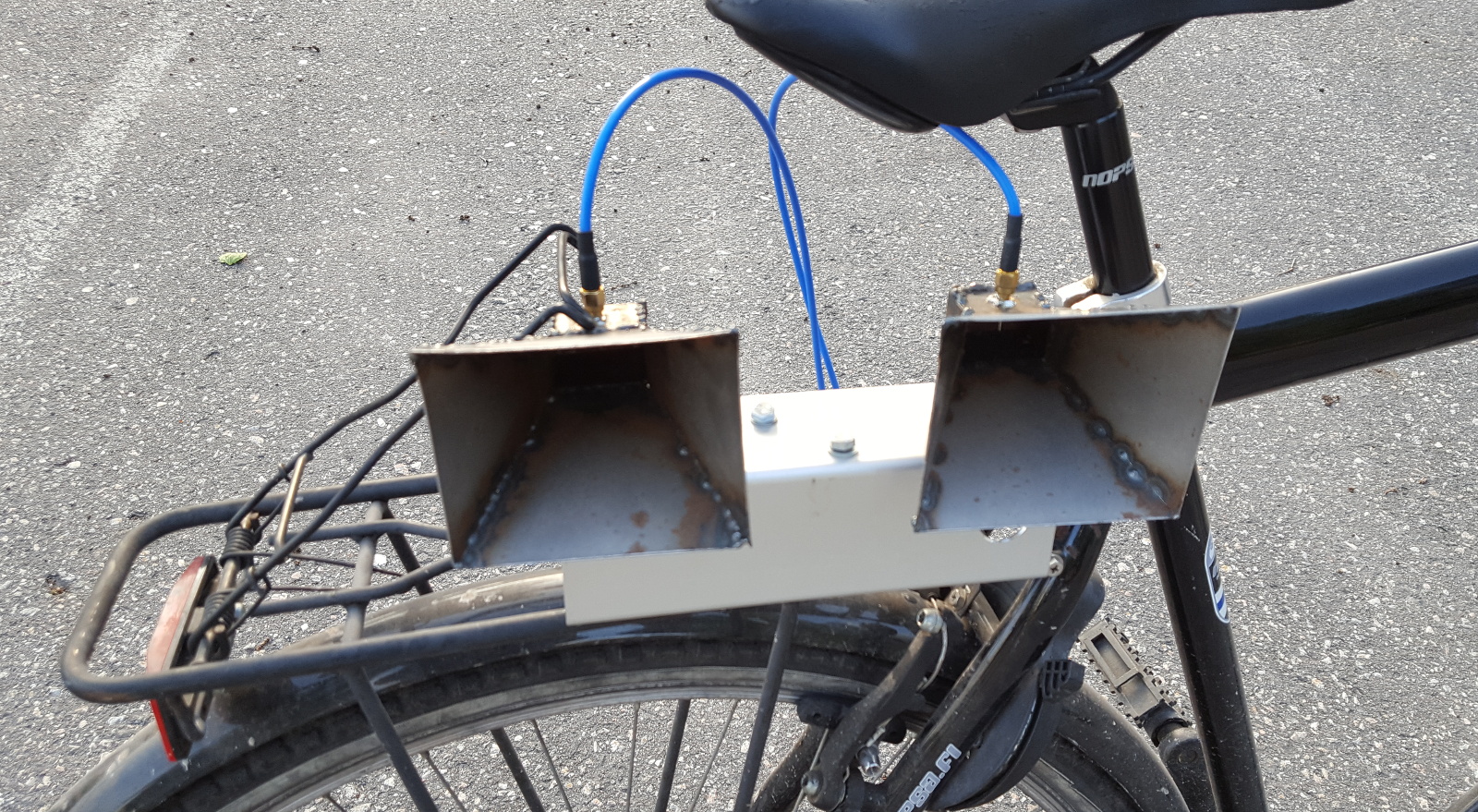
Radar mounted on the bicycle.
I mounted the radar on the rear rack of bicycle and pedaled the bicycle in a straight line with constant speed to take the measurement. It's very important that the path is known since any difference in the actual position and the one used during the image formation leads to image quality degradation. The position should be known within a fraction of wavelength to avoid any defocusing errors. My radar works at 6 GHz which works out to few cm precision requirement over about 200 m long path. This is probably not going to happen, but we are going to see later how the introduced position errors can be at least partly corrected.
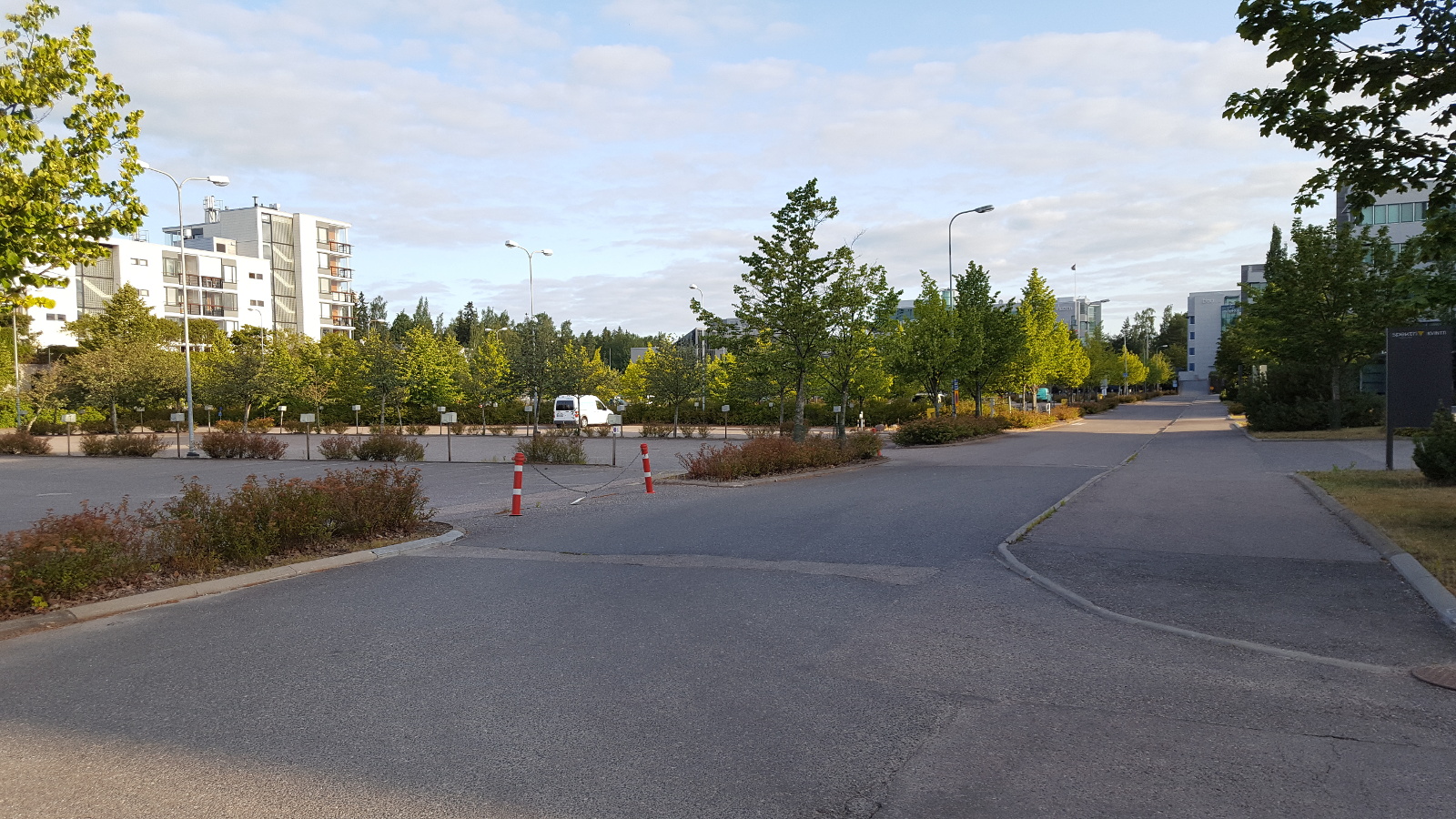
Photograph of the scene being imaged. Imaging path is on the footpath on right and the radar points to the parking lot on left.
In the above picture is the scene being imaged. It's a parking lot with lot of pole-like targets that should be well visible in the generated image.
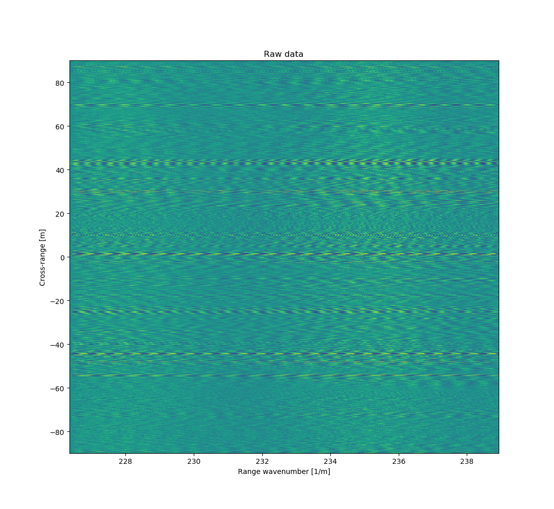
Raw data without any processing looks like this.
Raw captured data doesn't look like much. Sweep length is 1 ms, with 1 MHz sampling rate, so each sweep has 1000 points and there are total of 6444 sweeps. The output signal of the FMCW radar is a superposition of sine waves from each visible target. Frequency depends on the distance to the target, closer it is the lower the frequency. Amplitude depends on the amount of power reflected which depends on the size, shape, material and distance to the target.
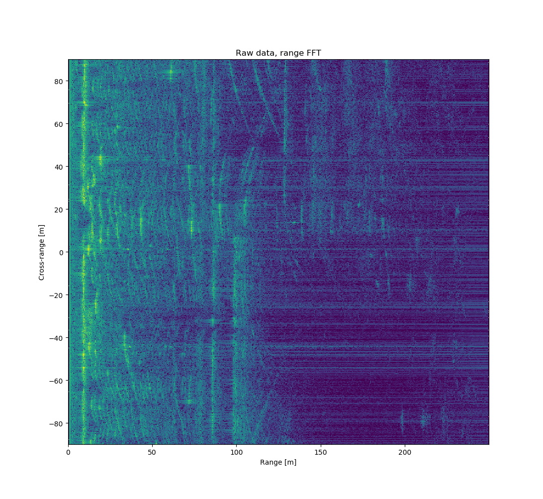
Taking FFT in range direction turns it into easier to read format with range on X-axis.
Above is FFT of the raw data in range direction. Range FFT is not part of the image processing, but this is how non-imaging measurement would be processed. FFT allows changing X-axis from wavenumbers to distance to the target.
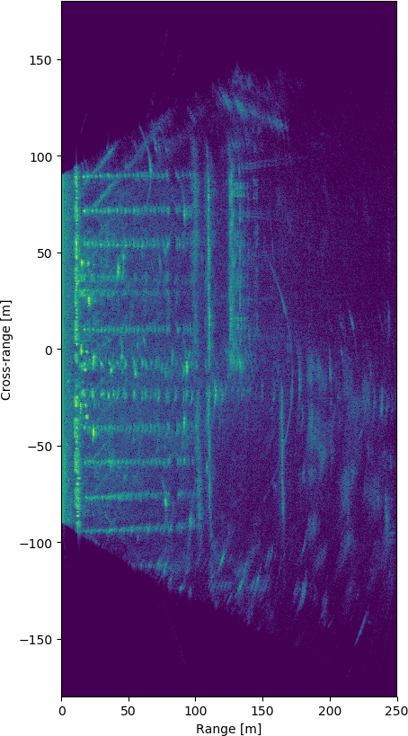
Running the Omega-k algorithm for the data generates the following image:
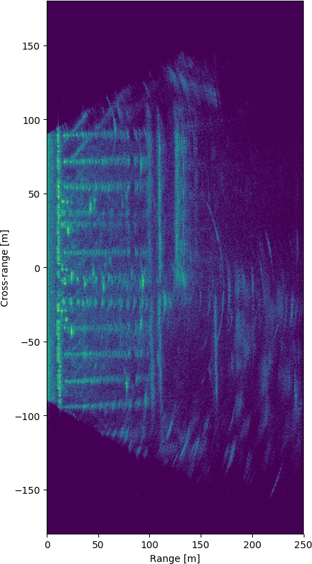
The image is mostly focused, there is some visible spreading but at least most of the targets can be recognized. There are some curved artifacts that I'm not sure where they come from.
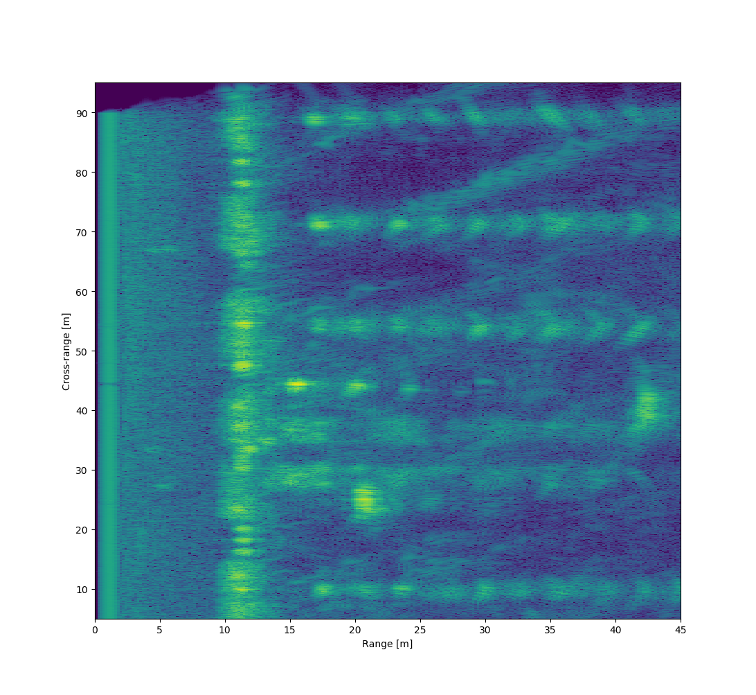
Generated SAR image of the parking lot. Zooming into the foreground.
When zooming into the foreground objects some smearing from movement deviations is visible. These can be fixed with autofocusing algorithm.
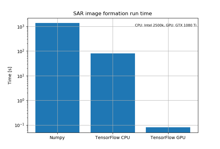
Image formation time on different programs using the above data from the parking lot. Program start-up and data preprocessing time is not included.
There is absolutely huge speed up from utilizing GPU. Numpy implementation does the FFT using Numpy and Stolt interpolation is coded in Python without vectorization. Numpy version takes 22 min and 30 s to form the image of the above data most of which is spent in the interpolation routine. TensorFlow CPU implementation calculates everything on CPU, Stolt interpolation is a custom op coded in C++. It is about 16x times faster than the Numpy implementation with most of the speedup coming from the much faster C++ interpolation function. Image formation takes 1 min 20 s.
TensorFlow GPU Python code is completely identical to the CPU version. It calculates FFTs using nVidia's cufft library on GPU and interpolation is done using custom CUDA kernel also on GPU. Image formation takes only 80 ms. The speedup is absolutely huge being over 1000x faster than TensorFlow CPU and over ten thousand times faster than the Numpy version.
Speedup from GPU shouldn't really be this much. I think part of the reason is that GPU implementation using nVidia's libraries is much more optimized than whatever CPU implementation TensorFlow uses. CPU FFT doesn't seem to be multithreaded, so just multithreaded FFT should speed it up by some small factor.
Minimum Entropy Autofocus
There are some inevitable motion errors when moving the radar on a bicycle. If there is a small deviation in direction of the antenna (Orthogonal to the movement path) it results in phase shifting the signal. If movement errors are known they can be corrected before the image formation by phase shifting the signal in the opposite direction by the equal amount. We don't know the errors but we can use TensorFlow to find the phase shift that minimizes some objective function that corresponds to how well the image is focused.
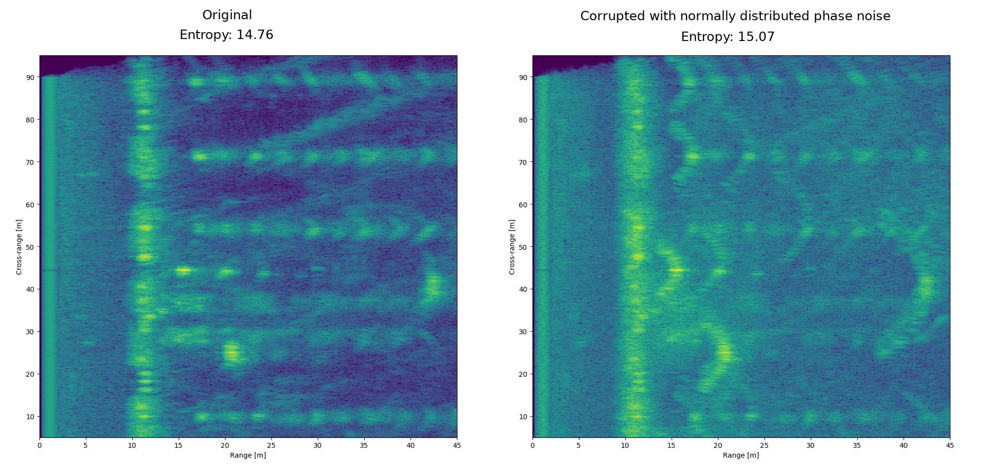
Comparison of the scene with and without added phase errors. The original scene that is visibly better focused also has lower entropy.
One objective function that corresponds with focusing of the image is entropy calculated as \(-\sum_{i} p_{i} \log(p_{i})\), where sum goes over all the pixels in image that is normalized so that all pixels sum to one and are in range \([0, 1]\).
Autofocus can be implemented simply in the code by phase shifting the measurement data at the beginning and adding optimizer that tries to minimize the entropy:
1 2 3 4 5 6 7 8 9 10 11 12 13 14 15 16 17 18 19 20 21 22 23 | |
Run the opt_op until the entropy has stopped decreasing and as a result we
should have found the phase errors that minimize the entropy. It's not very
efficient since this method requires running the image formation several times,
but since the GPU implementation is so fast it is not an issue.
I also found out that adding additional loss phase_smoothness that penalizes
large discontinuities in the phase results in slightly better quality image.
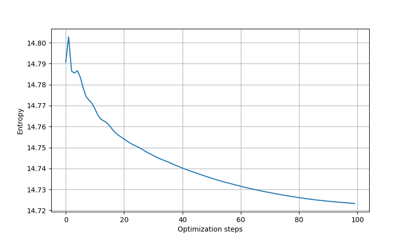
Entropy during the optimization.
I ran the optimizer for around 100 steps, more than that will still decrease entropy a little but there isn't really any significant visible changes in the image.
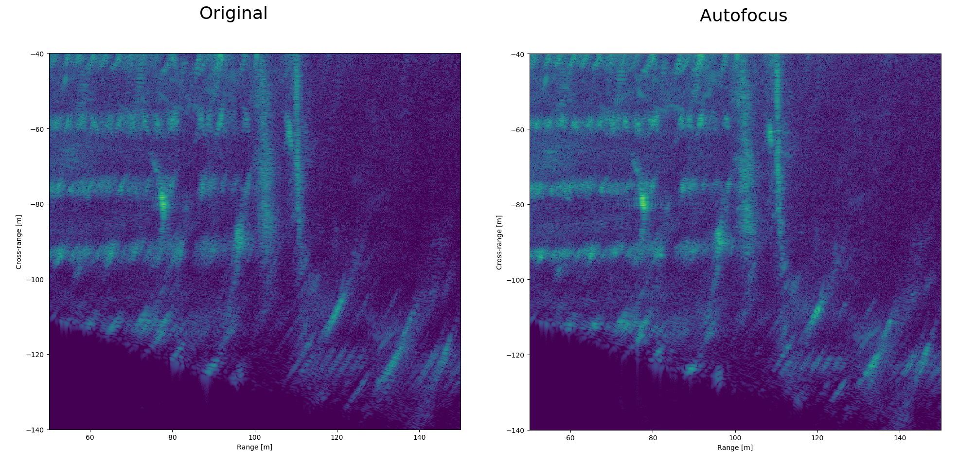
Autofocused image background compared to the original.
Difference between original and autofocused images is not huge, differences are mainly bigger around objects that are farther away and are illuminated for longer time.
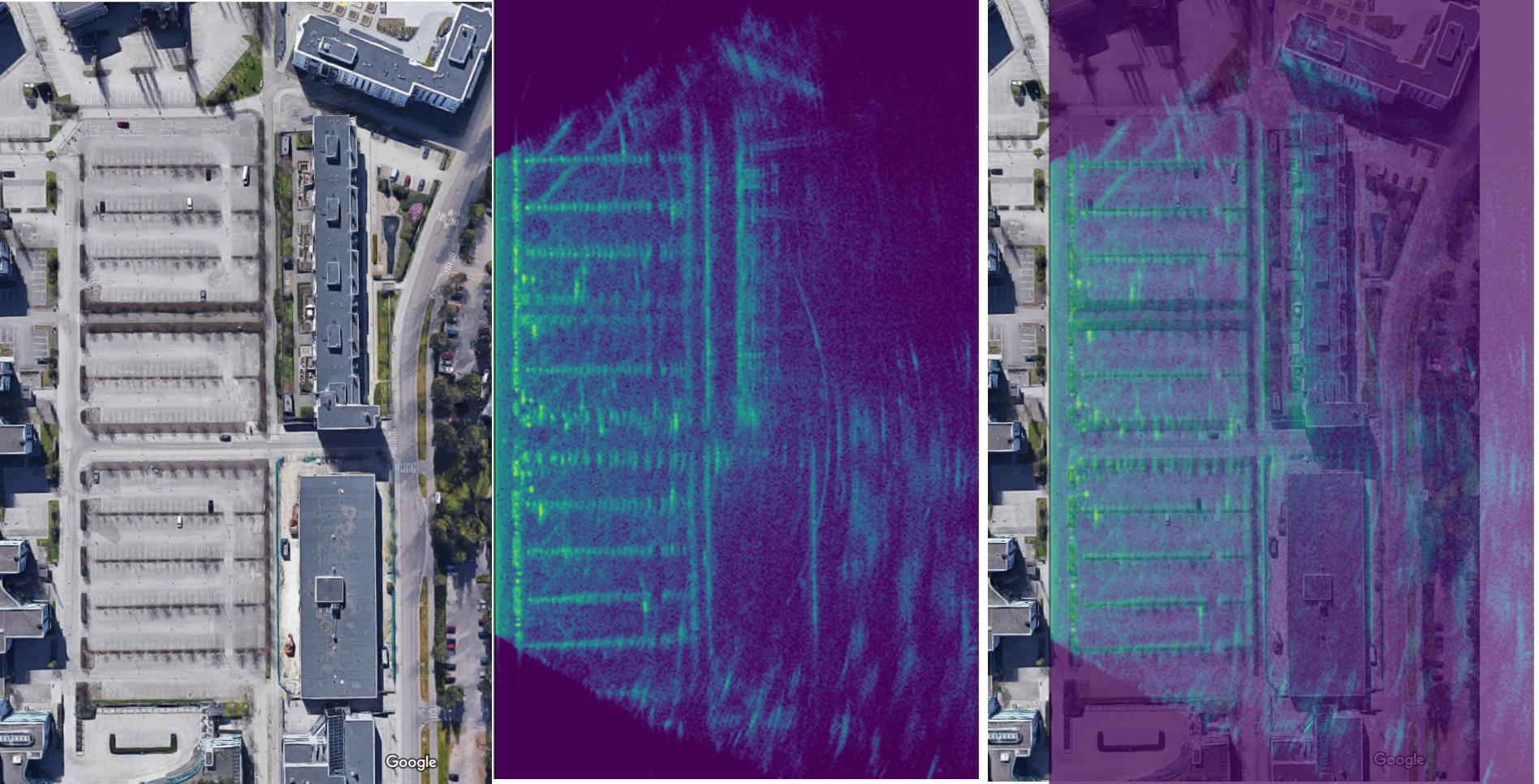
The generated SAR image matches pretty well with Google maps satellite image of the same location. Google data is slightly older and since it was taken the bottom building has been demolished. Cars are also obviously at different places.
Second scene
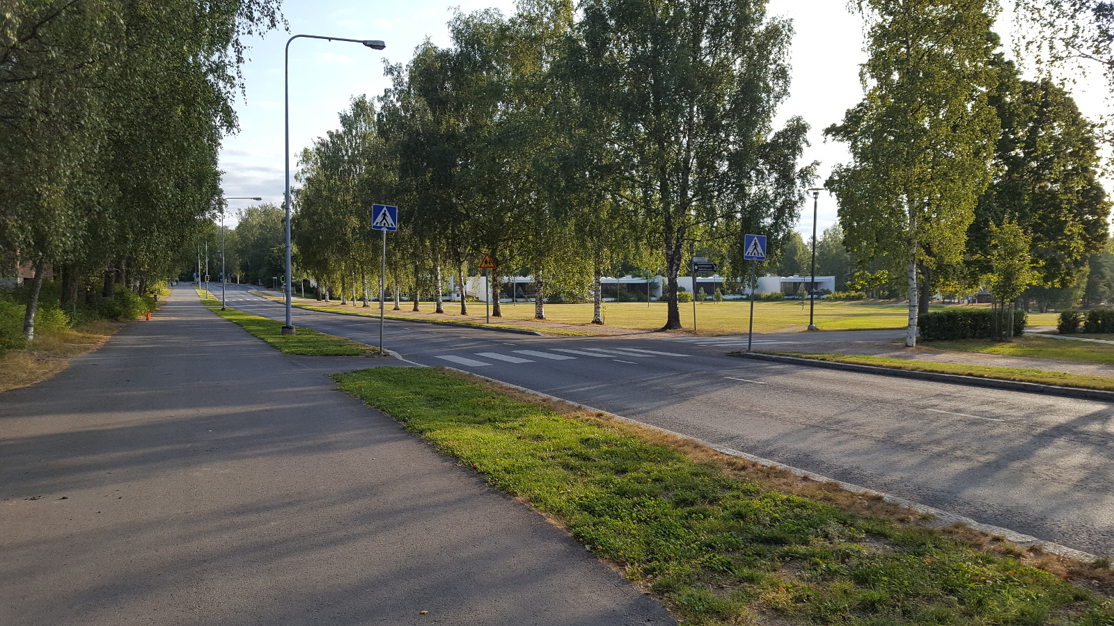
Photograph of the scene from the start of the track.
I also made measurements of a nearby park. There's a nice flat and smooth sidewalk next to it that allows easy measuring in a straight long line.

At the bottom there are some big buildings that occlude anything behind them. The reflection from them is large enough to saturate the receiver resulting in some artifacts. The light poles, street signs and trees on the foreground are very well focused, light poles very far away are spread a lot more. The problem with at least some of the farther away light poles is that they are occluded by other objects most of the time. The farthest light pole around 230 m is only visible for around quarter of the measurement time but even with that amount of observations it should still be sharper if the image was perfectly focused.
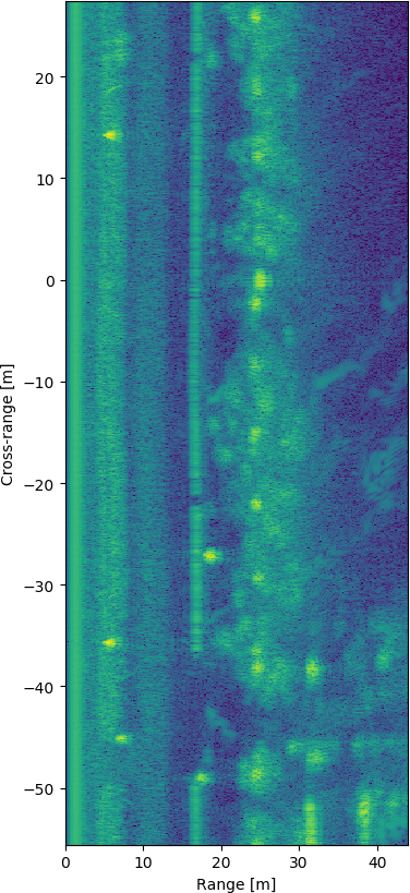
The foreground objects are well focused. Above are some objects that are also visible on the photograph above. The street curb is very reflective due to its shape. Grass and asphalt surfaces have slightly different radar reflectivity and the path to the zebra crossing is visible on the lower left corner.
The biggest issue is the inaccurate position information. Accurate velocity information should allow resampling the measured data to equal spacing and autofocus should take care most of the remaining sideways movement error.
Check out the code at GitHub or read how I made the radar hardware.