Introduction

This post is continuation of my previous synthetic-aperture imaging experiments. In the previous post I used omega-k frequency domain algorithm for the image formation and automatic differentiation based autofocusing with Tensorflow. I managed to get pretty well focused images from bicycle mounted radar considering the total lack of any motion recording data. The autofocus algorithm managed to improve it slightly, but it wasn't perfectly focused.

This time I'm implementing time-domain backprojection algorithm. It has slower $O(n^3)$ time complexity compared to $O(n^2\log n)$ of the omega-k, but it makes up for its slowness by its flexibility. Since omega-k is based on FFT it requires the data to be sampled on a straight line with equal spacing. However due to motion errors during the measurement this doesn't hold in practice. By adjusting the phase of the signal it's possible to approximate the signal that would have been recorded in slightly different position, but that approach has it's limits. Backprojection algorithm works with any shape measurement path.

Backprojection algorithm

Let's start the analysis of the algorithm with the radar signal model. My radar is frequency modulated constant wave (FMCW) radar that transmits short frequency sweeps. I won't repeat the derivation from the previous post, you can check it out if you want to see the details and I'll only give the resulting IF-signal for single target:

$$ s(n, \tau) = \exp\left(-j \frac{4 \pi}{c} (f_c + \gamma \tau) d(\mathbf{x}, \mathbf{p}_n)\right), \quad -T/2 < \tau < T/2 $$

, where $c$ is speed of light, $f_c$ is center frequency of the sweep, $\gamma = B/T =$ sweep bandwidth / sweep length $=$ sweep rate, $\tau$ is time variable and $d(\mathbf{x}, \mathbf{p}_n)$ is distance to the target at position $\mathbf{x}$ from the $n$th sweep at position $\mathbf{p}_n$.

Let's define discrete version of the IF-signal $s[n, m] = s(n, m T_s)$, where $T_s$ is the sampling interval.

The simplest way to generate a SAR image of radar measurements along some path is to use matched filtering. For each pixel in the output image it's possible to calculate what the measured IF signal would have been if there was a target at that pixel. Matched filtering the measured signal with the complex conjugate of the expected will give high value when the measurement matches the expectation. Repeating the filtering process for every pixel in the output gives the focused image. In equation form the filtering for one pixel can be written as:

$$ I(\mathbf{x}) = \sum_{n=0}^{N-1}\sum_{m=0}^{M-1} s[n, m] s_\text{ref}[n, m] $$

, where $s_{ref}[n, m]$ is the reference function which is complex conjugate of the expected IF response:

$$s_\text{ref}[n, m] = \exp\left(j\frac{4 \pi}{c}(f_c + \gamma m T_s) d(\mathbf{x}, \mathbf{p}_n)\right) $$

This SAR focusing algorithm gives especially well focused images, there are no interpolation steps, no approximations, it even works for cases where transmitter and receiver antennas are not at the same position. The big problem however is that it's extremely slow. For every pixel in the image it needs to go over every measured data point. For X x Y image and N sweeps each M points long the time complexity is in the order of $O(XYNM)$, or just $O(n^4)$ for short as they all scale linearly as the image size increases.

There is an easy way to speed it up with some slight assumptions about the measurement setup. If the reference function can be factored into two parts each depenging on only $n$ and $m$ then the double sum can be factored into two sums.

$$ I(\mathbf{x}) = \sum_{n=0}^{N-1} \exp\left(j\frac{4 \pi f_c}{c}d(\mathbf{x}, \mathbf{p}_n)\right) \sum_{m=0}^{M-1} s[n, m] \exp\left(j\frac{4\pi}{c} \gamma m T_s d(\mathbf{x}, \mathbf{p}_n)\right) $$

The trick for faster algorithm is using FFT to calculate the inner sum once and then using interpolation to index the right term for the outer sum.

The definition of the inverse FFT is: $S[n, k] = \sum_{m=0}^{M-1} s[n, m] \exp\left(j 2 \pi k m / M\right)$.

To solve for the right index into the FFT we need to solve for $k$ in the equation:

$$j 2 \pi k m / M = j\frac{4\pi}{c} \gamma m T_s d(\mathbf{x}, \mathbf{p}_n) $$

Solving for $k$ and using the fact that $\gamma = B/T$ and $T_s = T / M =$ sampling period gives:

$$ k = \frac{2 B}{c} d(\mathbf{x}, \mathbf{p}_n) $$

The backprojection algorithm can then be written as:

$$ I(\mathbf{x}) = \sum_{n=0}^{N-1} \exp\left(j\frac{4 \pi f_c}{c}d(\mathbf{x}, \mathbf{p}_n)\right) S\left[n, \frac{2 B}{c} d(\mathbf{x}, \mathbf{p}_n)\right] $$

, where $S[n, k]$ is the Fourier transform of $s[n, m]$ along the second axis. A slight complication is that the new index isn't necessarily a whole number and interpolation is required. The advantage of this form is that it completely removes the inner sum and replaces it with FFT calculated in advance. As a result time complexity of the algorithm improves from $O(n^4)$ to $O(n^3)$ and in practice the new form is much faster.

Bistatic correction

During this derivation it was assumed that transmitter and receiver antennas are at the same position, but that isn't exactly the case with my radar.

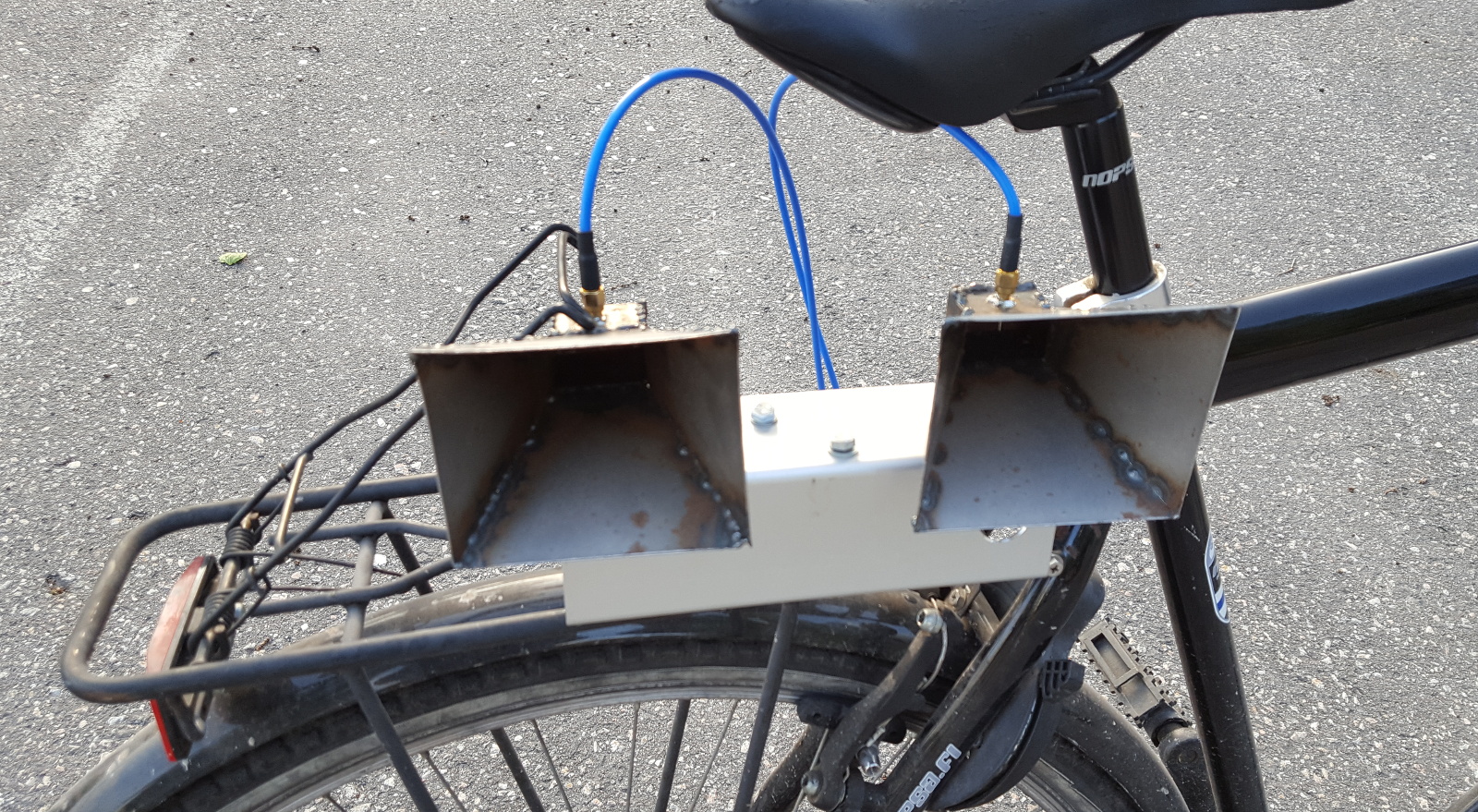
Radar mounted on the bicycle. Note the separate transmitter and receiver antennas.

As can be seen in the picture above I actually have separate transmitter and receiver antennas. While the error from considering them to be located on the same place isn't that large, it's not insignificant. Compensating for it in the Omega-k algorithm would have been very difficult, but it's trivial in backprojection algorithm. The distance that the radar measures is distance from transmitter antenna to target to receiver antenna. Replacing the distance to the target $p_n$ in the formula with average of distances from receiver and transmitter antennas to the target gives the measured distance.

Velocity correction

During the measurement the distance to the target is actually not constant due to movement of the platform. A correction for the movement was derived in the previous post for Omega-k and similar correction can be derived for the backprojection too.

First we assume that velocity is constant during one sweep, which isn't really unrealistic assumption as the acceleration would need to be absolutely enormous to have any difference in the speed during the short sweep. The second assumption is that velocity towards the target is constant during the sweep, this assumption is equal to only correcting for the first order errors of the velocity. In practice the non-linearity is so small with reasonable speeds that this isn't a large assumption.

Projection of the velocity $\mathbf{v}[n]$ to the distance vector gives the velocity component towards the target:

$$v_p[n] = \mathbf{v}[n] \cdot \frac{\mathbf{x} - \mathbf{p}_n}{\left|\mathbf{x} - \mathbf{p}_n\right|} $$

Distance to the target during the sweep can then be written as: $d(\mathbf{x}, \mathbf{p}_n) + v_p[n] m T_s$.

Substituting the new distance to the reference function gives:

$$ s[n, m] = \exp\left(j\frac{4\pi}{c}\left(f_c d(\mathbf{x}, \mathbf{p}_n) + \gamma m T_s d(\mathbf{x}, \mathbf{p}_n) + f_c v_p[n] m T_s + \gamma m^2 T_s^2 v_p[n] \right)\right)$$

The first two terms are the same as before, and the next two terms depending on $v_p[n]$ are new. The last term with $m^2$ dependence is problematic since it prevents writing the inner sum as FFT. Quadratic term could be ignored since it's typically much smaller than the other velocity term. By dividing the quadratic velocity term with the other term it can be shown that the quadratic term is at maximum $B / f_c$ of the other term. It mostly matters when sweep bandwidth is significant fraction of the operating frequency.

Better estimate than ignoring the quadratic term can be obtained by fitting a linear function to it (Stringham's PhD. thesis). Least square fit of linear function for $m^2$ over interval 0 to $M-1$ can be obtained by minimizing the sum below for $a$ and $b$:

$$ \min_{a,b}\sum_{m=0}^{M-1} \left(m^2 - (a m + b)\right)^2 $$

The solution can be found as $m^2 \approx (M - 1) m - \frac{1}{6} (M^2 - 3M + 2) \approx M m - \frac{M^2}{6}$.

Substituting it into the quadratic term and simplifying gives: $\gamma m^2 T_s^2 v_p[n] \approx \frac{\gamma m T^2 v_p[n]}{M} - \frac{1}{6} \gamma T^2 v_p[n]$

As before the reference function can be divided into two parts and the inner sum can be replaced with FFT:

$$ I(\mathbf{x}) = \sum_{n=0}^{N-1} \exp\left(j\frac{4 \pi}{c} \left(f_c d(\mathbf{x}, \mathbf{p}_n) - \gamma T^2 v_p[n]/6\right) \right) S\left[n, \frac{2 B}{c} \left(d(\mathbf{x}, \mathbf{p}_n) + \frac{f_c v_p[n]}{\gamma}\right) + T v_p[n]\right] $$

In the outer exponential $4\pi\gamma T^2 v_p[n]/6c = 4\pi B T v_p[n] / 6c$ is normally small enough to be ignored.

The difference to the case where radar was assumed to be stationary during the sweep is just a slight adjustment to the index of the $S[n, k]$.

Tensorflow implementation

Implementation of the backprojection was made as a custom operation in Tensorflow with both CPU and GPU support. The algorithm is excellent candidate for GPU implementation as the parallelization is straightforward: each pixel in the image can be calculated independently. Interpolation needed in the indexing of the FFT result is implemented as simple linear interpolation. FFT is calculated with configurable amount of zero-padding to smooth the output and make the interpolation result more accurate. The result is acceptable even with this simple interpolation unlike interpolation in Omega-k algorithm where linear interpolation would cause visible artifacts in the image.

For calculating gradients, a gradient operation also needs to be implemented. Specifically operation calculating the chain rule needs to be implemented. The operation takes as input the accumulated gradient from the earlier gradient operations and calculates the gradient at the inputs of the operation.

Gradients of complex numbers need some care in Tensorflow. Gradient of real function $y(x)$ with respect to $x$ is calculated simply as $\frac{\partial y}{\partial x}$, but the formula is different if the function is complex valued. The short version is that the gradient of complex valued function $f(x)$ with respect to $x$ needs to be calculated as $\overline{\left(\frac{\partial f}{\partial x} + \frac{\partial \overline f}{\partial x}\right)}$, where $\overline \cdot$ is complex conjugate. For more detailed explanation see this discussion. In this case the second term, conjugated partial derivate, is zero and the result is the normal real gradient but conjugated. For simplicity velocity correction terms are ignored but adding them is trivial. Using chain rule gradient of the backprojection for one pixel of output can be calculated as:

$$\frac{\partial I(\mathbf{x})}{\partial \mathbf{p}} = \sum_{n=0}^{N-1} \frac{\partial d(\mathbf{x}, \mathbf{p}_n)}{\partial \mathbf{p}} \exp\left(j\frac{4 \pi f_c}{c}d(\mathbf{x}, \mathbf{p}_n)\right) \left( j\frac{4 \pi f_c}{c} S\left[n, \frac{2 B}{c} d(\mathbf{x}, \mathbf{p}_n)\right] + \frac{2 B}{c} \frac{\partial S}{\partial d(\mathbf{x}, \mathbf{p}_n)}\left[n, \frac{2 B}{c} d(\mathbf{x}, \mathbf{p}_n)\right] \right)$$

The gradient computation needs gradient of $S$. In the forward direction linear interpolation was used to calculate the values in between the sample points and it's natural to use the slope of the linear interpolation to define the necessary gradient.

The gradient operation calculating the chain rule is complex conjugate of the above gradient times the accumulated gradient summed over all the pixels in the image. If $E$ is some scalar output of the graph and $g$ is the accumulated gradient from all the operations after the SAR image formation, the gradient of $E$ with respect to the input positions can be written as:

$$ \frac{\partial E}{\partial \mathbf{p}} = \sum_\mathbf{x} g[\mathbf{x}] \overline{\left(\frac{\partial I(\mathbf{x})}{\partial \mathbf{p}}\right)}$$

Autofocus

With the backprojection and its gradient operation implemented using Tensorflow for autofocusing the generated image is easy. First calculate the SAR image and it's entropy. Entropy of image generally correlates with how focused image is with better focused images having lower entropy. Next calculate gradient of entropy as function of the input position vector using automatic differentation. A small step towards negative gradient vector should decrease the entropy improving the focus of the image. The steps are repeated until entropy doesn't decrease anymore.

In practice there are some slight issues with the above algorithm. If position of every sample can be optimized individually there are too many degrees of freedom. There are many positions for the samples that give a focused image with low entropy, but most of them have some geometric distortions that don't correspond to the actual scene. For example adding any position offset to all of the samples just moves the resulting image. Backprojection algorithm requires specifying the pixel coordinates beforehand and without any constraints the optimizer can just add a large offset to every sample to move all the data out of the scene to minimize the entropy. Some constraints need to be added for the sample positions to make sure that the optimized image makes sense. Almost all SAR data is taken on a straight path with constant velocity, so it's natural to add some constraints to keep the positions close to a straight line with equal spacing.

Autofocused parking lot image with geometric erorrs due to unrestriected sample positions. There is a kink in the image near origin that shouldn't be there.

In the above image is an example of the scene with unrestricted position optimization. The image looks focused but it has severe geometric distortions as the parking spaces should be evenly spaced. See pictures at the bottom on how the image should look like.

I added two extra constraints for velocity. The first adds penalty if the range direction of the velocity is too large and other adds penalty if the azimuth velocity difference to its mean value is too large. With these constraints the geometric errors are avoided in the cases I tested.

Focusing data With 6444 sweeps each with 1000 samples each for 9666 x 1933 pixel output image the FFT based Omega-k takes 56 ms for one forward iteration and backprojection algorithm takes 436 ms. The time-domain backprojection algorithm is almost ten times slower on this dataset but compared to the Omega-k algorithm it's much more flexible. Omega-k algorithm requires the transmitter and receiver to be at the same position and all samples to be recorded on a straight line with equal distance in the direction of movement between them. Time-domain backprojection can focus any kind of measurement configuration with possibly unevenly samples positions and non-colocated transmitter and receiver antennas.

Measurements

For good comparison with the Omega-k algorithm I focused the previously measured data also with the backprojection algorithm. Autofocus was run for 100 iterations.

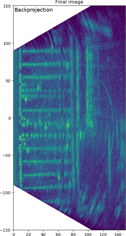
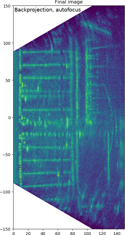
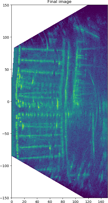
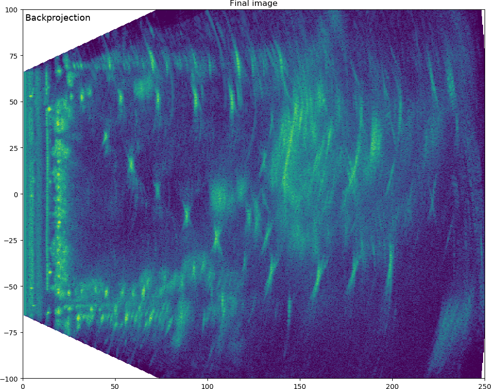
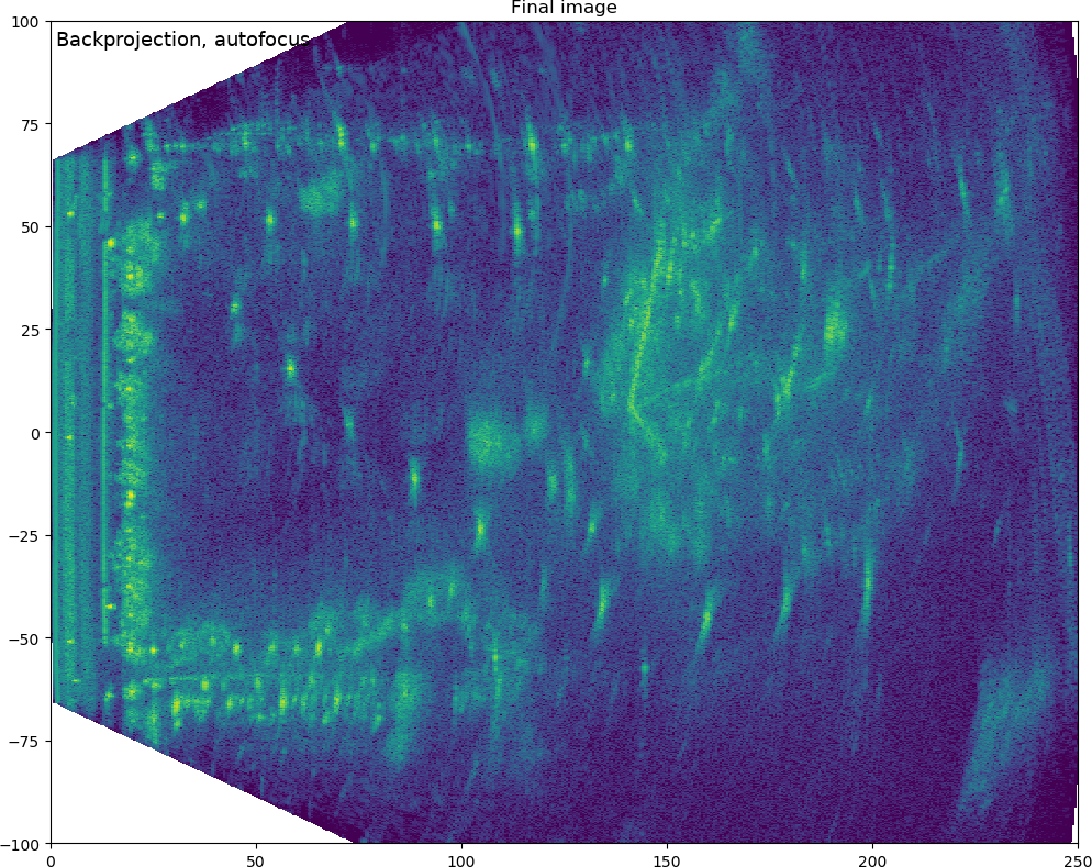
Parking lot scene SAR image. Click/tap to see the autofocused version.

Above is the image of the parking lot from the same data as I previously used for the Omega-k algorithm post expect that the sampling rate is twice as large as before avoiding some aliasing artifacts from before. Clicking/tapping and holding shows the focused image. The difference the autofocus makes is big and the autofocused image has excellent focusing.

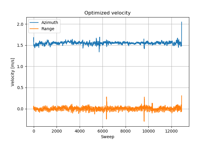
Solved velocity

The solved velocity is almost constant, there are small oscillations in the range direction and some slight variance in the azimuth direction. There are some spikes that correspond to locations where there are large objects that saturate the receiver. This method doesn't seem to give the best results when receiver has saturated, some spreading of the big objects can be seen as a result in the image.

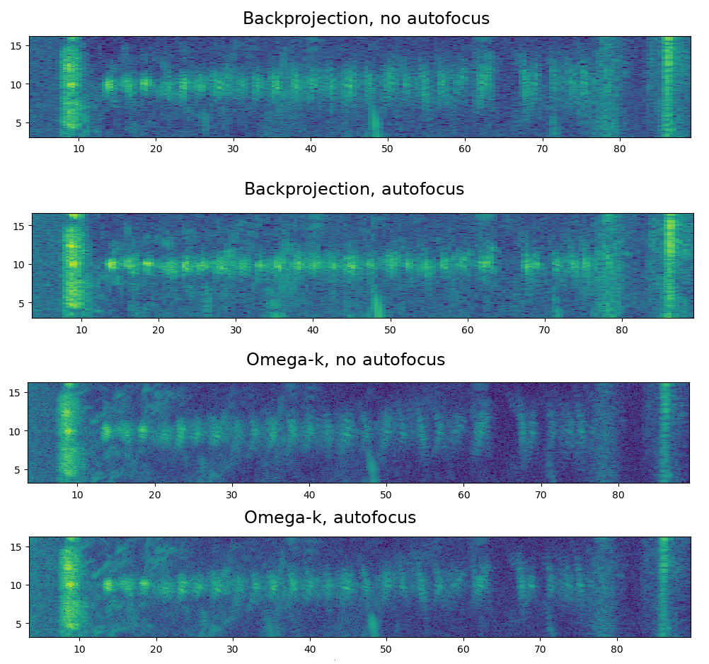
Comparison of backprojection and omega-k with and without autofocusing.

For farther away objects the difference in focusing between the algorithms is big. In the above comparison image both autofocus algorithms improve the focusing for nearby targets, but only backprojection with autofocusing can also focus the farther away targets.

Park scene SAR image. Click/tap to see the autofocused version.

I also redid the other scene I measured the last time. The improvement from autofocus in that scene is also huge especially for objects farther away. The objects farther away are still spread, but I'm not sure if they should be much better than what they are now. There are lot of issues with occlusions in this scene and some far away objects are visible for the radar only for a very short time. See the images in the previous post for the same data focused with Omega-k algorithm.

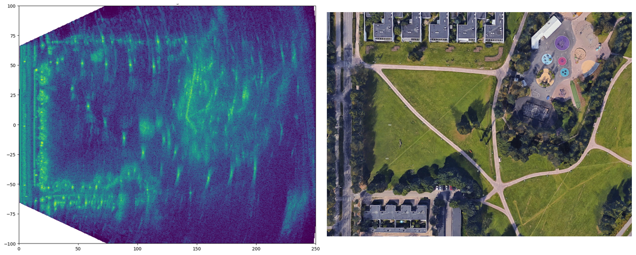
Comparison to Google maps image of the same location.

Light posts and tree trunks are very visible in the SAR image compared to the Google maps image. Most of the details inside the park in the upper right can't be seen in the SAR image since a metal fence blocks the most of the view from the radar signal.

Conclusion

I implemented a fast GPU based time-domain backprojection algorithm for synthetic aperture radar image focusing with autofocus based on automatic differentiation implemented as custom operation in Tensorflow. The autofocus algorithm gives a big improvement to focusing of the data from my homemade radar without any position measurement. The code is available at my Github.