Introduction
A radar with one transmitter and one receiver antenna can measure distances to the targets based on the time of flight of the transmitted electromagnetic wave. One transmitter and receiver isn't however enough to measure angle in which the targets are. A simple way to get the angle information is to use antenna with a very narrow beam and mechanically rotate it. Mechanical rotation does have some drawbacks. It requires a large antenna to achieve the narrow beamwidth, rotating the large antenna requires lot of space and the whole field of view can't be imaged at the same time.
Instead of rotating a single antenna, a radar with multiple stationary antennas can be used to generate image of the targets. Phased array radars use multiple antennas to form the radar image without needing to physically rotate. Because the antennas can operate at the same time the image refresh rate is much faster. MIMO radar is phased array radar with multiple transmitter and receiver antennas. The more antennas are used the better the angular resolution of the radar.
I have been working with MIMO radars for few years. When I started I didn't know much about them and there didn't seem to be much of introduction level material at the time. Many of the existing material in my opinion are overly complex and don't give good intuition about the subject. This post is my try to make introduction level article about the MIMO radar antenna array design that I wished I had when I started to design MIMO radars.
Antenna array beamforming basics
Radar works by transmitting electromagnetic waveform from the transmitter antennas which reflects from the targets and is received by the receiver antennas. Based on the time delay between transmission and reception the distance to the target can be calculated. This doesn't give any information about the angle where the object is. To know the angle of the target multiple antennas are needed. The antennas are at slightly different locations and thus receive the signal at slightly different times. Based on the time differences at each antenna the angle of the target can be solved. In practice instead of the absolute time difference, which would required extremely good time resolution, phase of the received signal is used.

Distance of the traveled radar waveform.
If we assume that the target is very far and the angle to the target from each antenna can be assumed to be identical then the distances the radar waveform travels to each antenna is summarized in the above figure. We will also make another assumption that the distance difference to the target between the antennas is less than range resolution of the radar. This assumption simplifies the image formation as all signals will be in the same range bin after the image formation.
The distance traveled by the radar waveform is the distance from TX antenna to target plus distance from the target back to the RX antenna: \(r_{tx} + r_{rx1} = 2r_{tx} + d\sin \theta\). With multiple receiver antennas at different distances to the transmitter the radar waveform travels slightly different distance which can be used to solve for the angle of the target.
The received signal from one target at the RX antenna is of the form: \(f_{\text{rx}} = A f_{rx0}\exp\left(\frac{2\pi j}{\lambda} d\sin \theta\right)\). \(A\) is the amplitude of the received signal, \(f_{rx0}\) is the time-delayed transmitter waveform that would have been received at the transmitter antenna. Exponential term is phase shift that depends on the distance to the target \(r\) and wavelength of the radiated signal \(\lambda = \frac{c}{f}\). Complex numbers are used to make the analysis mathematically simpler, the actually measured signal are of course real valued and only the real part of the expression would be measured.
With one target and two receiver antennas at different distance the angle of the target can be easily determined by comparing phase differences of the received signals at the two receiver antennas. The phase difference of the received signals at two antennas at distances \(d\) and \(2d\) from the transmitter is \(\exp\left(\frac{2\pi j}{\lambda} d\sin\theta\right)\), angle of the target \(\theta\) can be easily solved from the expression. For there to be a single solution the distance \(d\) needs to be less than \(\lambda/2\), otherwise due to periodicity of \(\sin\) same phase could be obtained at two or more angles.
Multiple targets
The situation is a little bit harder when there are multiple targets. Reflection signals from the different targets sum at the receiver and only the summed signal can be measured. With one target the amplitude of the signal was the same at all antennas, but with multiple targets this is not necessarily the case.
After the radar waveform \(f_{rx0}\) is demodulated from the receiver signals, each receiver's output is of the form \(f_{rx,n} = A_n \exp{j \phi_n}\). Matched filtering is the optimal linear filter to determine how likely it is that there is a target at each angle. In this case the matched filter is the signal that would be observed from a single target at the particular angle: \(g_n(\theta) = \exp\left(\frac{2\pi j}{\lambda} d_n\sin\theta\right)\).
The target distribution \(t(\theta)\) can be calculated as:
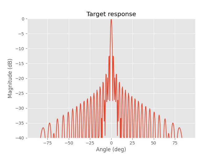
Setting \(f_{rx,n} = 1\) we get the target response of a single target at zero angle.
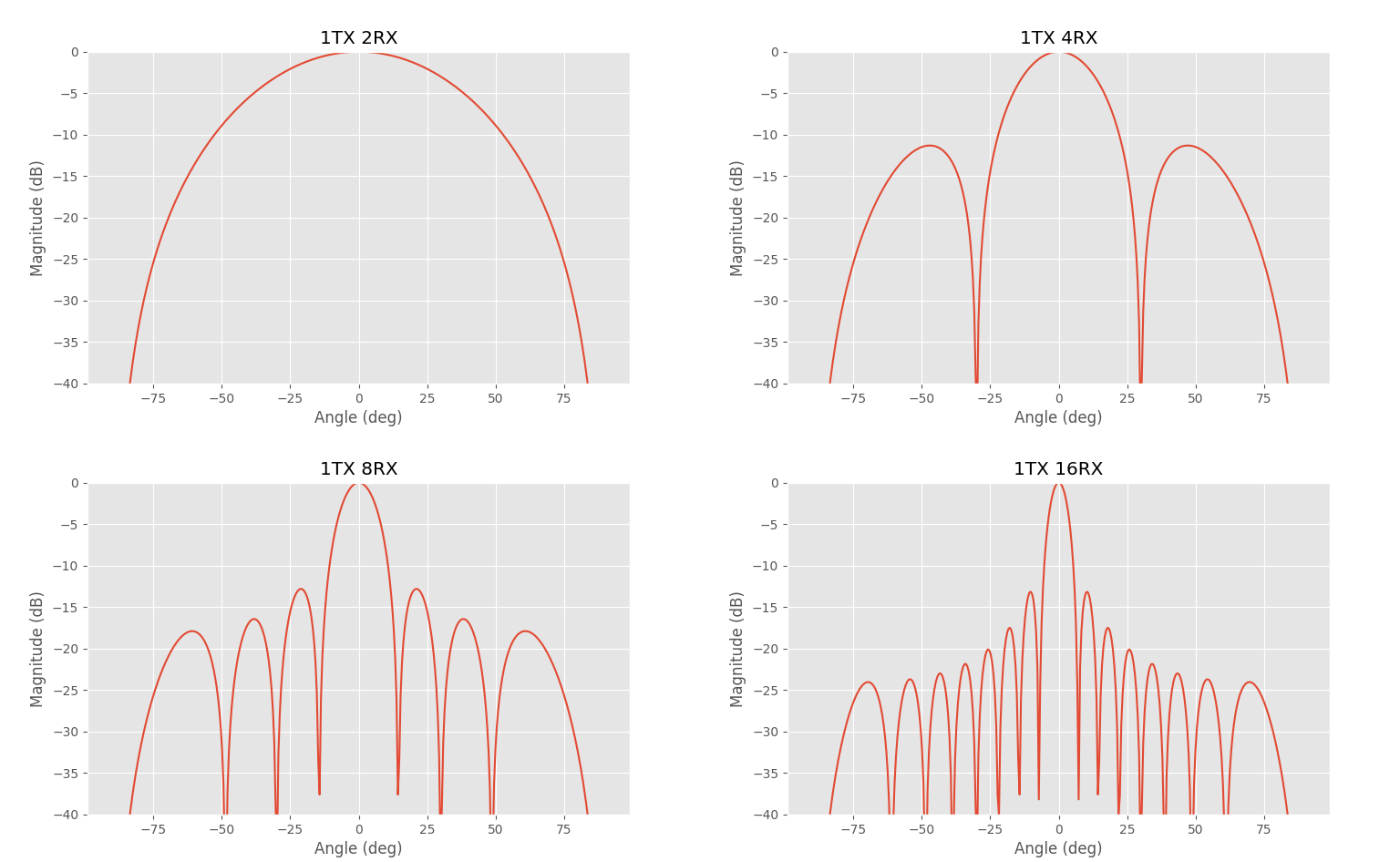
Antenna array detected target response with different number of RX antennas. Half wavelength spacing.
In the above figure are some target responses with arrays having single transmitter and different number of receivers. Many antennas are required to get a decent angular resolution. Even with 16 receivers the -3 dB angular resolution is just 6 degrees.
Sidelobe level could be adjusted by weighting the terms in the sum. Without weighting the first sidelobes are at -13 dB level.
Antenna arrays with multiple transmitters
For the MIMO principle to be possible we need to assume that receivers can separate the signals from different transmitters. If they would transmit at the same time the same waveform they would just sum up at the receivers and they can't be separated. In practice the transmitters could transmit at different times, at different frequencies or the waveforms are orthogonal and correlator at the receiver can separate them.

Two transmitters and two receivers.
The above antenna configuration is similar to the previous one with one transmitter and two receivers, but now a second transmitter has been added at distance \(2d\). The TX1-RX1 and TX1-RX2 signals are the same as before and there are also additional TX2-RX1 and TX2-RX2 signals. We can write \(r_{tx2}\) as a function of \(r_{tx1}\) and distance between the transmitters \(2d\) as \(r_{tx2} = r_{tx1} - 2d\sin\theta\). The distance from TX2 to target to RX1 can be written as: \(r_{tx2} + (r_{tx1} + d\sin\theta) = 2r_{tx1} - d\sin\theta\). Writing the distances to target of all pairs gives the following table:
| Antenna pair | Traveled distance |
|---|---|
| TX2-RX1 | \(2r_{tx1} -d\sin\theta\) |
| TX2-RX2 | \(2r_{tx1}\) |
| TX1-RX1 | \(2r_{tx1} + d\sin\theta\) |
| TX1-RX2 | \(2r_{tx1} + 2d\sin\theta\) |
1TX-4RX array
The 2TX-2RX array with four antennas gives identical length differences between the antenna pairs to 1TX-4RX array with five antennas in the above figure. This results in the identical formed radar image. If the TX2 antenna was moved to the same position as RX2 the measured lengths would match perfectly to the 1TX-4RX array. The constant offset in the measured distances doesn't matter for determining the target angle and I didn't draw it like that because figure would have been not as clear.
Using two transmitters we have saved one total antenna. The savings are even bigger with bigger arrays. MIMO array makes independent measurement for each TX-RX pair, while antenna array with only one transmitter can make measurements equal to the number of receiver antennas. For example with 32 receivers and 32 transmitters each TX-RX pair gives independent measurement for total of 32*32 = 1024 measurements. Antenna array with only one transmitter would need 1024 receiver antennas to get the same number measurements and achieve the same angular resolution.
Virtual transceiver array
In the last section 2TX-2RX array was found to behave similarly to 1TX-4RX array when the antenna spacing were as given. If the antenna spacings would have been different they would not have matched. Antenna arrays with a single transmitter are easy to analyze. The problem is how to determine the correct antenna spacings of the MIMO array to match regular antenna array?
To ease the analysis of MIMO arrays it's possible to calculate virtual element positions of the antenna array. Each virtual element is an overlapping transmitter and receiver that only receives its own transmitted signal. This virtual transceiver antenna array is easier to analyze. In practice for each TX-RX pair we place a virtual transceiver antenna at half way between the both antennas.

TX-RX pair and virtual antenna at half-way between them.
In the above picture is a TX-RX pair at distance \(d\) and a virtual element half way between them. The TX to target to RX distance is \(2r_{tx} + d\sin\theta\). Distance from virtual element to target to virtual element is \(2(r_{tx} + \frac{d}{2}\sin\theta) = 2r_{tx} + d\sin\theta\), which is equal to the TX-RX pair.
One important detail about the transceiver elements is that while regular antenna array spacing needs to be less than half wavelength to avoid aliasing, transceiver element spacing needs to be less than quarter wavelength. This is because transceiver element has both transmitter and receiver overlapping. Moving the transceiver element by quarter wavelength away from the target changes the distance to the target by half wavelength.
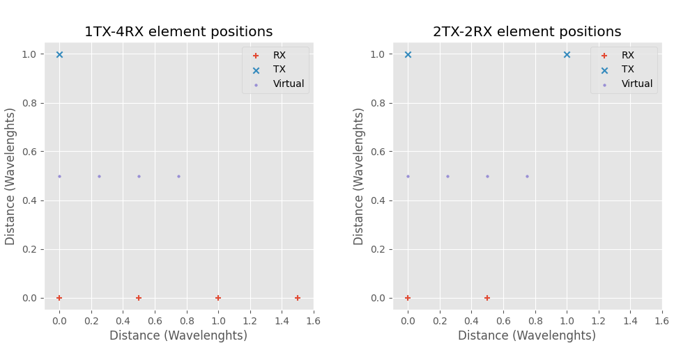
1TX-4RX and 2TX-2RX antenna arrays with virtual elements.
In the above picture are 1TX-4RX and 2TX-2RX array antenna locations with the virtual elements marked. Despite having smaller physical size and less antennas virtual element places are identical to the 1TX-4RX array.
2D MIMO antenna arrays
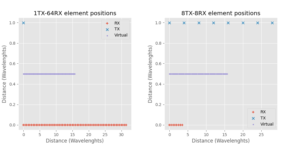
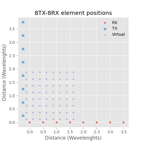
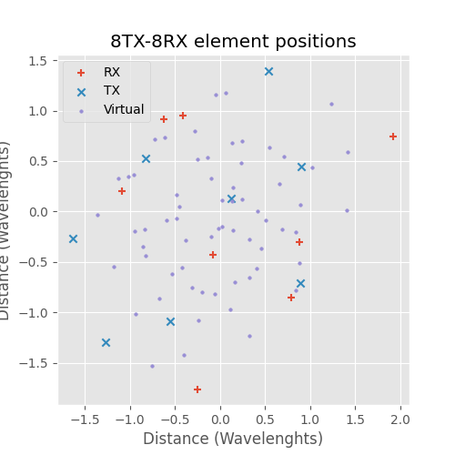
1TX-64RX and 8TX-8RX antenna arrays.
In the above figure 1TX-64RX and 8TX-8RX arrays are compared. 8TX-8RX MIMO array has less less antennas, is physically smaller and has the same virtual array as the 1TX-64RX array. 1TX-64RX physical size is 31.5 wavelengths, 8TX-8RX size is sligthly smaller 28 wavelengths. The Y-axis TX to RX distance is arbitrary and doesn't have effect on the target detection. Target response at zero angle is plotted below.
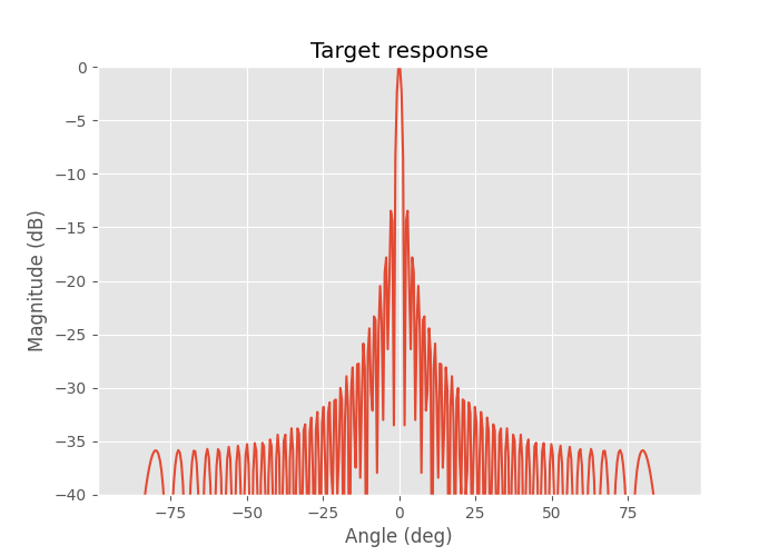
64 virtual element with λ/4 spacing target response at zero angle.
The angular resolution is about 1.6 degrees which starts to be a decent resolution for a radar.
However there is another MIMO array configuration that results in the same virtual array but is physically even smaller. The trick is to split the RX array in two and put them in the opposite sides of the TX array.
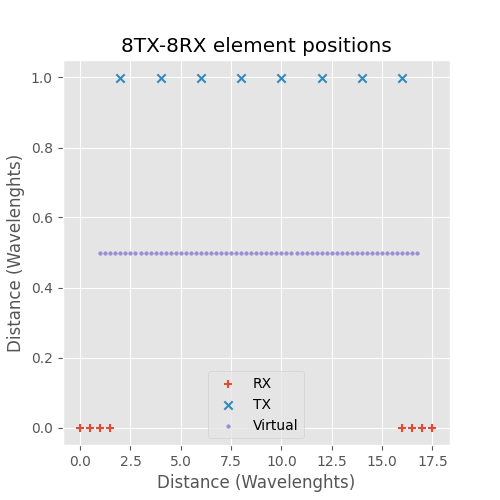
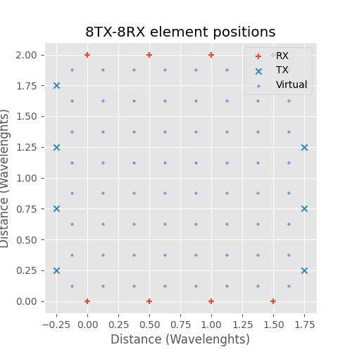
8TX-8RX split RX MIMO array.
The 8TX-8RX MIMO array in the above figure results in the exact same virtual array as the two previous arrays, but the physical size is much smaller at only 17.5 wavelengths. This is almost two times smaller than 1TX-64RX array and in fact as the number of elements increases the split RX MIMO array takes only half of the space of equal array with one transmitter.
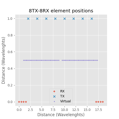
There are also other possible 8TX-8RX MIMO arrays that have the same virtual array, but they are not as compact as the split RX array. However they might be useful in some situations. In the figure below is one example:
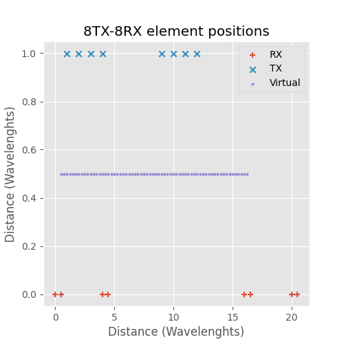
Alternative 8TX-8RX RX MIMO array.
3D MIMO antenna arrays
Previously the antenna arrays have been one dimensional linear arrays, the obtained radar image has distance and azimuth angle to the target. They were called 2D arrays as the radar image is 2D and has no inclination angle (target height) component. To obtain the also the inclination angle and the full 3D position of the targets the antenna array needs to be two dimensional.
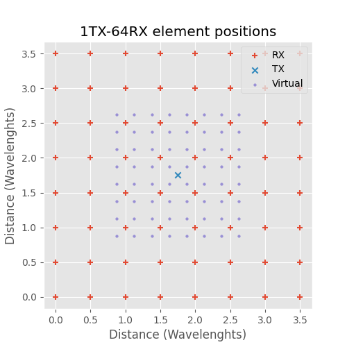
Dense 1TX-64RX 3D antenna array.
With one transmitter the receivers need to be arranged in a dense grid in this case 8x8 requiring total of 64 receiver antennas.
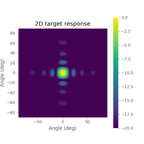
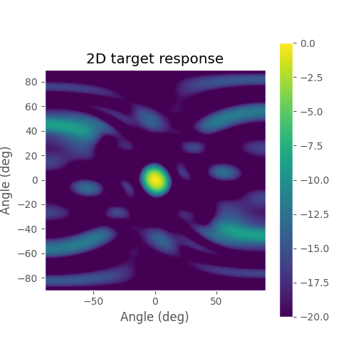
Target response of 1TX-64RX 3D array.
The angular resolution is not that good since there is only eight antennas for X and Y directions.
One MIMO array that has the same virtual array can be achieved by arranging TX and RX antennas in perpendicular rows:
8TX-8RX MIMO 3D antenna array.
While this requires less total antennas it doesn't save space. Similar to split RX 2D array the splitting of the antennas can be done with the 3D array to achieve a box shaped array:
8TX-8RX MIMO 3D box antenna array.
The virtual element array is the same as before but now the physical size is smaller. Similarly to the 2D case, as the number of elements increases the side dimensions of box shaped MIMO array are half of the dense receiver array with one transmitter.
The box configuration does have one drawback that in the corners TX and RX antennas need to be very close together, the distance is only 0.35 wavelengths. In practice this can cause issues with large TX-RX coupling.
The box array has a nice property that it can be tiled while still achieving dense virtual element spacing without any gaps or overlapping elements:
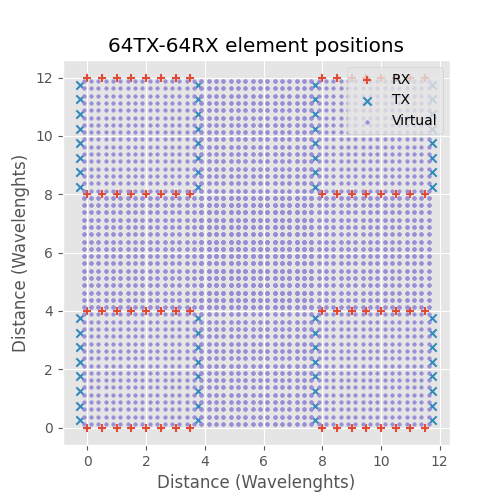
Four tiled 8TX-8RX MIMO 3D box antenna arrays.
This is very useful in practice as it gives space to place components in a large array and allows manufacturing the large array with smaller modules.
Non equally spaced MIMO arrays
All of the above arrays resulted in equally spaced virtual array. This is very useful property in practice as it allows using Fast Fourier Transform in the image formation greatly speeding it up. However non-equally spaced array is also possible and it's possible to calculate their responses with the same equations.
8TX-8RX MIMO array with wider split RX spacing.
If the antennas are not at exactly the right places the virtual array won't be uniform.
Target response of the above array.
Larger absolute size of the virtual array leads to narrower main lobe, but gaps in the virtual array increase the side lobe levels.
Randomly placed 8TX-8RX MIMO array.
In the above picture 8TX and 8RX antennas were placed randomly in -2 to +2 wavelength box following uniform distribution.
Target response of the above array.
Characteristic of randomly distributed antennas is narrow main lobe but high side lobe level.
Receiver antenna virtual array
It's possible to also make virtual array of only receiver antennas. In that case virtual element positions are sum of position of each pair instead of average when using transceiver elements. This kind of virtual array is usually more common for example in text books. It doesn't matter which one is used when analyzing the far field radiation pattern, but one case where it makes a difference is MIMO SAR (synthetic aperture array). MIMO SAR virtual array can be calculated by sum of individual virtual arrays only if transceiver elements are used. I also think that transceiver array derivation is mathematically cleaner.
Conclusion
MIMO radar array with \(N_{tx}\) transmitters and \(N_{rx}\) receivers can achieve angular resolution comparable to antenna array with one transmitter and \(N_{tx} N_{rx}\) receivers. With the right antenna distribution MIMO array can be made half the size of regular antenna array while still achieving the same angular resolution.
The code for visualizing the antenna arrays is available here.