Introduction

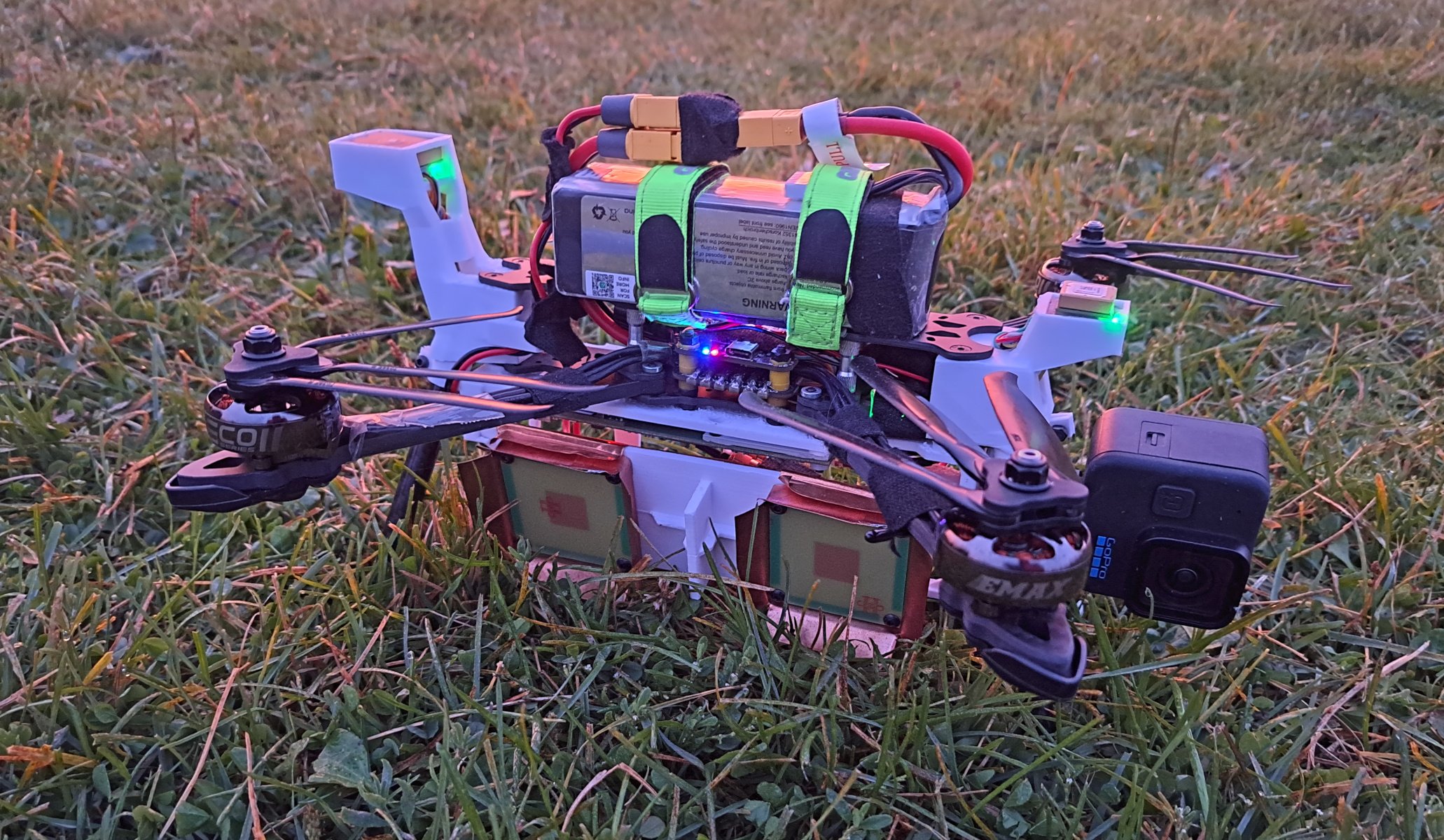
Radar drone. Since the first post I have added a Gopro camera and a second GPS for redundancy.

Earlier this year I made a polarimetric synthetic aperture radar (SAR) mounted on a drone. I have since worked a lot on the software side to improve the image quality and now the same hardware can generate much better quality images. The main contribution of this article is description of a new SAR autofocus algorithm that combines some of the existing SAR autofocus algorithms to make an algorithm that is well-suited for drone mounted SAR. Also antenna pattern normalization and polarimetric calibration suitable for drone mounted SAR with non-linear track is described.

Radar signal

SAR image formation geometry.

While the drone flies along a track, the radar measures the distances and phases of the targets in the antenna beam. Neither azimuth ($\varphi$) nor elevation ($\theta$) angle of a target can be determined from a single measurement, and all targets at the same range will overlap in the measurement. However, by recording many radar measurements from multiple locations, a radar image can be formed.

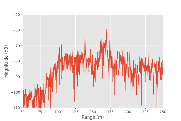
Magnitude of a single recorded range compressed radar signal.

Depending on the radar parameters and radiated waveform, the signal processing to obtain a range-compressed signal from the raw recorded data might vary. After range compression, however, the image formation process is essentially the same.

Range resolution is the ability to separate two closely spaced targets. Ideally it's calculated as $\Delta r = c/2B$, where $c$ is speed of light, and $B$ is the bandwidth of the radiated waveform. For example, with a 150 MHz bandwidth the range resolution is 1 m. For a linear flight track this is also the image resolution in range direction.

The phase of the received signal depends on the distance to the target. Because the signal travels to the target and back, a distance change equal to half the wavelength causes a full wavelength (360 degrees) shift in the received signal phase. As a function of target distance, the phase can be written as $\varphi = 4\pi d/\lambda$, where $d$ is distance, and $\lambda$ is wavelength. For instance, with 6 GHz RF frequency, a distance change of 25 mm (1 inch) causes 360 degree phase shift.

SAR image formation

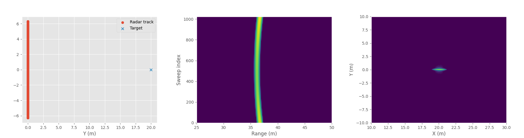
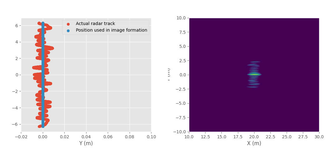
SAR image example with one point target. Radar track and target position (left), magnitude of the recorded radar data at each position (middle), and processed SAR image (right). Platform height is 30 m.

Due to the wide antenna beam there are multiple targets in the beam at the same time, but with signal processing it's possible to separate them and generate much higher resolution image.

To convert a set of radar measurements into a radar image, matched filtering can be used. For each pixel in the image grid, generate a reference signal corresponding to what a target at that position would reflect. For each radar measurement, multiply the measured signal with complex conjugate of the reference signal, then sum these products over all measurements. When the measured signal closely matches the reference signal, their product becomes large because the phases align and target is generated at that location in the image. If the phases don't match, the result of the multiplication is a complex number with a random phase, and summing random complex numbers will average out generating a low response and that pixel in the image will have low amplitude.

Assuming the signal is already range compressed and ignoring the amplitude (antenna pattern and loss due to distance can be compensated after image formation), then the reference signal just needs to compensate for the phase.

The image formation can be written as:

$$I = \sum_{p \in \mathcal{P}} \sum_{n=1}^N S_n(d(\mathbf{p},\mathbf{x_n})) \exp \left(j \frac{4\pi}{\lambda} d(\mathbf{p},\mathbf{x_n})\right)$$

$\mathcal{P}$ is the set of pixels in the image, $N$ is the number of radar measurements, $S_n$ is range compressed single channel radar measurement, and $d(\mathbf{p},\mathbf{x_n})$ is the distance to location of pixel $\mathbf{p}$ from radar position at measurement $\mathbf{x_n}$.

Position error

To get a well focused radar image, the phase of the reference signal used in the matched filtering needs to match with the recorded signal. If there is any error in the actual position of the radar during measurement to the position used in image formation, it will cause errors in the image.

Assuming the target is just a single point and ignoring the amplitude, with $\Delta \mathbf{x_n}$ position error on the $n$th measurement, the error in image at the location of the target can be calculated as:

$$I_p = \sum_{n=1}^N S_n(d(\mathbf{p},\mathbf{x_n})) \exp \left(j \frac{4\pi}{\lambda} d(\mathbf{p},\mathbf{x_n} + \Delta\mathbf{x_n})\right) = \sum_{n=1}^N \exp \left(-j \frac{4\pi}{\lambda} d(\mathbf{p},\mathbf{x_n}) + j \varphi_p\right) \exp \left(j \frac{4\pi}{\lambda} (d(\mathbf{p},\mathbf{x_n} + \Delta\mathbf{x_n})\right)\\ = \sum_{n=1}^N \exp \left(-j \frac{4\pi}{\lambda}\left(d(\mathbf{p},\mathbf{x_n}) - d(\mathbf{p},\mathbf{x_n} + \Delta\mathbf{x_n})\right) + j\varphi_p \right) = \sum_{n=1}^N \exp \left(-j \frac{4\pi}{\lambda}\Delta r_{n,p} + j\varphi_p\right) $$

Instead of all phases lining up at the location of the target, there is some phase offset left that depends on how the position error changes the distance. The remaining error $\Delta r_{n,p}$ is the distance error from $n$th radar position to the target location at pixel $p$.

$\varphi_p$ is a constant phase offset from the target. It can be caused by phase change in reflection, small position offset or just phase offset in the radar electronics.

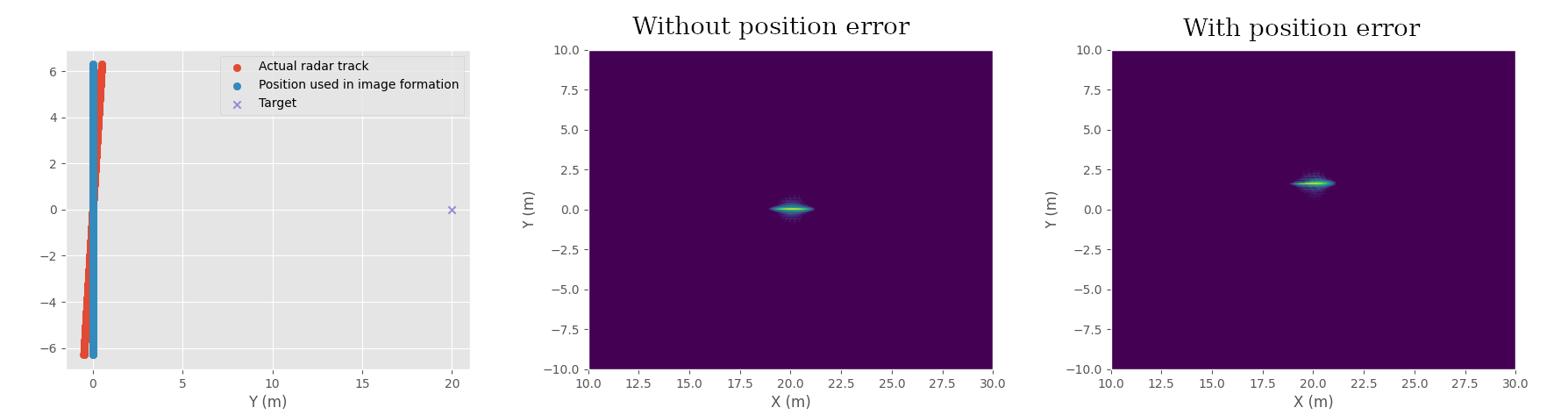
SAR image example with one point target, with and without linear error in radar position. Radar track and target position (left), image processed without position error (middle), and image processed with linear position error (right) causing shift in the image.

SAR track can have any shape, but often it's a straight line. With this simple track it's possible to calculate how some position errors affect the image.

If the distance error $\Delta r_{n,p}$ is constant, then the error is just a constant phase offset which doesn't affect the magnitude of the image at all.

Linear error affects the image by shifting the azimuth positions of the targets in the image. Analysis for it is in many different papers and textbooks, but a good detailed overview can be found in the paper: "Performance Limit of Phase Gradient Autofocus Class Method for Synthetic Aperture Radar" by C. Tu, Z. Dong, A. Yu, Y. Ji, X. Chen and Z. Zhang.

The same scene, but with more complicated position error. Radar track and position error (left), and image processed with position error (right) causing blurring of the target.

More complicated errors can be thought as piecewise linear error, each piece in the position error causes the resulting image to be formed at different location resulting in a blurred image.

Note the scale of the position error that causes the blurring in the simulate image. The maximum error is only 1 cm, but even this small error causes significant loss in the image quality. Since the image formation relies on the phase, position error must be much smaller than wavelength to not cause phase errors during image formation. In this case the simulation uses 6 GHz RF frequency which corresponds to 5 cm wavelength.

Generalized phase gradient autofocus

The idea behind autofocus algorithms is to estimate the error in radar position from the SAR image and radar data. There are many different autofocus algorithms for different applications, but the most widely used SAR autofocus algorithm is phase gradient autofocus (PGA). The generalized version isn't as well known and was published much later, but in my opinion it's easier to understand with backprojection image formation background.

To simplify the notation let's call the terms used for calculating a single pixel $I_p$ in backprojection $\xi_{n,p}$:

$$\xi_{n,p} = S_n(d(\mathbf{p},\mathbf{x_n})) \exp \left(j \frac{4\pi}{\lambda} d(\mathbf{p},\mathbf{x_n})\right)\\ I_p = \sum_{n=1}^N \xi_{n,p}$$

The idea behind phase gradient autofocus is that if we know that a target in the SAR image is a point target, then phase of $\xi_{n,p}$ should be constant. If this is not the case, the position error can be solved from the $\xi_{n,p}$ by finding a phase offset that makes it constant. The phase error can then be converted to distance to find the position error.

$\xi_{n,p}$ is calculated exactly like a pixel in the backprojection image formation but just without summing up the terms.

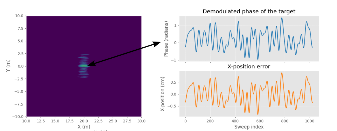
SAR image with position error (left) and phase of ξ calculated at the target location compared to position error.

Calculating the demodulated target phase ($\xi_{n,p}$) for the previous example scene gives a phase that matches very well with the X-position error that was added to the radar position. Shifting the phase of the input data by negative of the $\xi_{n,p}$ would result in a constant phase, which results in a focused target in the image.

In this case since the target is on X-axis the distance error is very close to the X-axis error, but this is not the case generally if the target is at some other angle. A more general method for solving for the 3D position error from the phase error will be presented later.

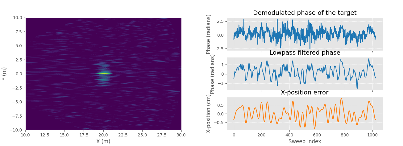
Low-pass filtering will improve the phase error estimation when phase error is slowly varying. SAR image with noise and position error (left) and demodulated phase of the target with and without low-pass filtering (right).

Low-pass filtering is used to filter out noise and clutter at the same distance in measurements as the target. Since the target response is a constant it will be preserved as the signal is low-pass filtered, but any noise and other objects that were momentarily at the same distance as the target being considered are filtered out. Low-pass filtering also filters out high frequency position errors if it's too small, so the low-pass window size should be set carefully.

Low-pass filtering operation is often implemented as Fourier transforming the signal, zeroing the high frequency bins, and then inverse Fourier transforming to get the filtered signal.

GPGA algorithm flow-chart. Algorithm is iterated until either phase error is below a threshold or minimum low-pass filter window size is reached.

The complete GPGA algorithm needs few more operations. In general there are many point-like targets in the same image and for the best position error estimation multiple different targets should be used.

We know that for a point target with position error: $\xi_{n,p} = \exp(-j\frac{4\pi}{\lambda}\Delta r_{n,p} + j\varphi_p)$.

The constant phase offset, $\varphi_p$, that is different for each target makes it impossible to just sum different $\xi_{n,p}$ for each target together. There are few different phase estimators for estimating the phase error from set of $\xi_{n,p}$ from many targets (pixels $p$).

One solution is to calculate:

$$g_{n,p} = \xi_{n-1,p}^* \xi_{n,p} = \exp\left(j\frac{4\pi}{\lambda}\Delta r_{n-1,p} - j\varphi_p\right) \exp\left(-j\frac{4\pi}{\lambda}\Delta r_{n,p} + j\varphi_p\right) = \exp\left(-j\frac{4\pi}{\lambda}(\Delta r_{n,p} - \Delta r_{n-1,p})\right)$$

Multiplying complex conjugate of n+1th term with nth term causes the constant phase to cancel out and the result is a difference in phase errors between adjacent positions (phase gradient in the algorithm name). In this forms the $g_{n,p}$ from different targets can be summed, taking the argument of the sum gives the gradient of the phase error, and the phase error can be recovered up to a constant phase offset by calculating a cumulative sum.

$$g_n = \text{Arg} \left(\sum_{p} g_{n,p}\right)$$

In practice the sum should be weighted according to signal-to-clutter ratio in each target response for the optimal estimate and this weighting will be analyzed later. Finally taking cumulative sum of the phase gradient $g_n$ gives estimate for the phase error.

After correcting the image with the solved phase error, the phase error is reduced but might not be completely gone. Decreasing the low pass window size and repeating the process improves the estimate.

3D trajectory estimation

So far only the phase error has been solved. It can be used to correct the SAR image by multiplying the input data with the negative of the phase error. However, the phase error is proportional to distance error from the radar position to the target, and depending on a target's location, the phase error caused by the position error varies. If several targets at different azimuth and elevation angles are visible at the same time, it might not be possible to focus them all at the same time with a single phase-correction term. This is the case when antenna beam is wide, which is precisely the case with my drone mounted SAR.

Example scenario with two targets and 2D position error. Distance errors to the two targets are not equal due to their different azimuth angle. r1' is about equal to r1 due to direction of the position error being mostly perpendicular to target 1, but this is not the case for target 2. There isn't a single phase correction that will focus them both at the same time.

To get all the targets in focus at the same time it's necessary to solve the 3D position error and use the corrected position of the radar during the image formation.

The 3D trajectory estimation is based on paper "An Autofocus Approach for UAV-Based Ultrawideband Ultrawidebeam SAR Data With Frequency-Dependent and 2-D Space-Variant Motion Errors" by Z. Ding et al. The first step is to divide the SAR image into $K$ subimages and then calculate the phase error in each image using PGA or GPGA. The phase error can be turned into a distance error by unwrapping the phase and multiplying by $\lambda/4\pi$. The result is distance error from each radar position ($N$ positions) to each subimage ($K$ subimages).

GPGA can solve for distance error to each local image and the 3D position error can be solved from multiple distance errors to different subimages.

If the subimages are small, we can assume that azimuth and elevation angle to all the targets in the subimage are similar and use the weighted target positions as the subimage center position. At this point we have a distance error from each radar position to each subimage. The number of subimages is large and we only have three unknowns (x, y, and z position errors), and we can set up an overdetermined system of equations to solve for the 3D position error from the distance errors and known subimage center positions.

Calculating the 3D position error from distance errors to each subimage would require solving a non-linear system of equations due to distance calculation not being linear, but assuming that 3D position error is small it can be linearized which makes solving it much easier and faster.

Knowing the subimage center azimuth and elevation angles, the distance error $\Delta r_{n,k}$ from $n$th radar position to $k$th subimage center can be written as a 3D Cartesian vector: $[\Delta r_{n,k} \cos \theta_{n,k} \cos \varphi_{n,k}, \Delta r_{n,k} \cos \theta_{n,k} \sin \varphi_{n,k}, \Delta r_{n,k} \sin \theta_{n,k}]^T$, where $\varphi_{n,k}$ is azimuth angle from $n$th radar position to $k$th subimage center ($0$ to $2\pi$) and $\theta_{n,k}$ is elevation angle ($-\pi/2$ to $+\pi/2$), note that this is different from the usual spherical coordinate definition that uses inclination. Assuming that $\Delta r_{n,k}$ is small then the target azimuth and elevation angles are almost the same before and after the shift and the linear system for solving the 3D position error at $n$th position can be written as:

$$\mathbf{R_n} = \mathbf{M_n} \Delta \mathbf{x_n}$$

$$\mathbf{M_n} = \begin{bmatrix}\cos \theta_{n,0} \cos \varphi_{n,0} & \cos \theta_{n,0} \sin \varphi_{n,0} & \sin \theta_{n,0} \\ \cos \theta_{n,1} \cos \varphi_{n,1} & \cos \theta_{n,1} \sin \varphi_{n,1} & \sin \theta_{n,1}\\ ... & ... & ...\\ \cos \theta_{n,k} \cos \varphi_{n,k} & \cos \theta_{n,k} \sin \varphi_{n,k} & \sin \theta_{n,k} \end{bmatrix}, \, \mathbf{R_n} = \begin{bmatrix}\Delta r_{n,0} & \Delta r_{n,1} & ... & \Delta r_{n,k}\end{bmatrix}^T, \, \Delta \mathbf{x_n} = \begin{bmatrix} \Delta x_n & \Delta y_n & \Delta z_n \end{bmatrix}^T$$

$\mathbf{M_n}$ is a Kx3 matrix of subimage center angles, $\mathbf{R_n}$ is Kx1 matrix of distance errors to each subimage, and $\Delta \mathbf{x_n}$ is 3x1 matrix of 3D position errors.

Solving the linear system for $\Delta \mathbf{x_n}$ at each radar position gives the desired 3D position error.

Weighted Least Squares

In a real SAR image signal-to-clutter ratio can vary a lot between different targets. To get the most accurate estimate measurements should be weighted by the signal-to-clutter ratio. The calculation for approximate of the signal-to-clutter ratio from the target demodulated phase is quite involved and the full details can be found in paper: "Weighted least-squares estimation of phase errors for SAR/ISAR autofocus" by Wei Ye, Tat Soon Yeo and Zheng Bao.

The final result is that weighting factor $w_p$ for each target in GPGA can be written as:

$$w_p = \frac{1}{\sigma_p^2} = \frac{d}{4 c^2 - 2d - 2 c \sqrt{4 c^2 - 3 d}}$$

$$d = E(|g_{n,p}|^2),\, c = E(|g_{n,p}|)$$

Weighting factor equals $1/\sigma_p^2$ which is the inverse of variance of the phase error in the measurement from target $p$. This weight should be used to weight each target in GPGA phase gradient estimation.

In 3D trajectory estimation the weighting factor is the combined weight of all targets in the subimage. It can be calculated as:

$$w_k = 1 / \sum_{p} 1 / w_p$$

GPGA 3D trajectory deviation estimation

GPGA algorithm with 3D trajectory deviation estimation.

Putting it all together the algorithm is quite computationally demanding due to multiple image formations required. They could be skipped in some cases, but the best performance is obtained when a new image is formed after every iteration to get a better estimate of true target locations. However, when using fast factorized backprojection it's quite fast when implemented on GPU even with a large amount of data.

Compared to other autofocus algorithms I believe this is one of the most general ones. It computes the 3D position error, it doesn't assume linear track and can work with any shaped flight track, it can correct for position error that exceeds range resolution, it works with digital elevation model, and it can be extended to work with 3D imaging SAR or bistatic SAR systems.

I implemented the algorithm on GPU using custom CUDA kernels and despite it's heavy computation requirement it runs very quickly. In practice even just few iterations result in a large improvement in image quality and it's much more efficient than the Minimum entropy autofocus that I previously used.

The code is open source and available as "gpga_bp_polar_tde" function in torchbp package.

Synthetic example

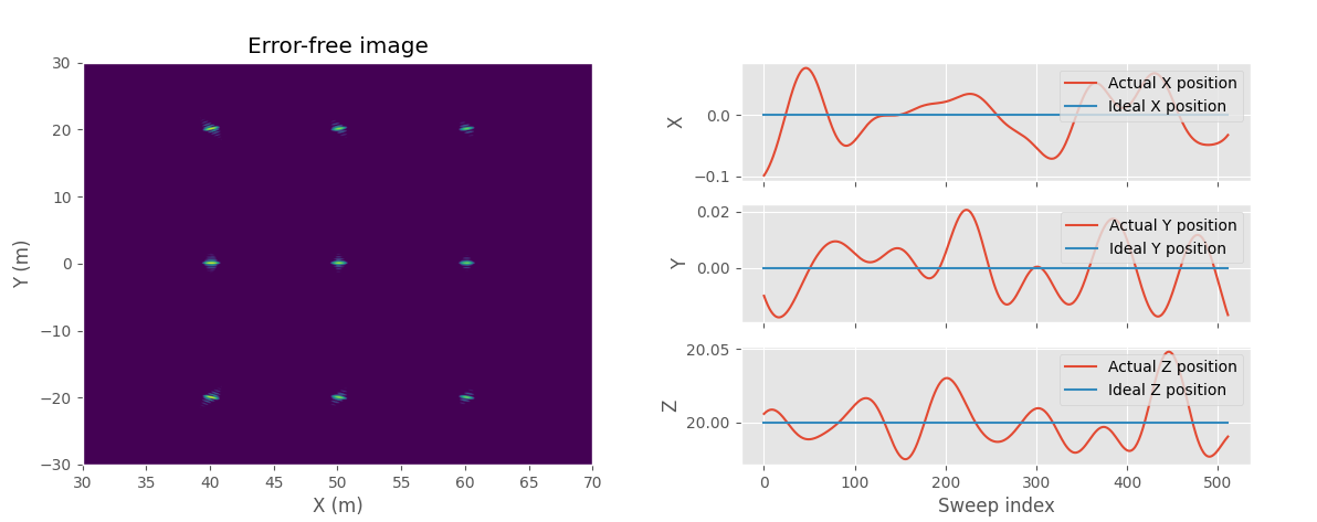
Ideal SAR image of the point targets without any position error (left). Position error added to the image (right), Y-axis linear trend is removed.

I made a small synthetic example with nine point targets in a grid. The height of the radar was set to 20 m and it moves linearly along Y-axis sampling every quarter wave length (12.5 mm / 0.5 inch). I added random low frequency 3D position error to the radar position and used the corrupted position to form the initial SAR image.

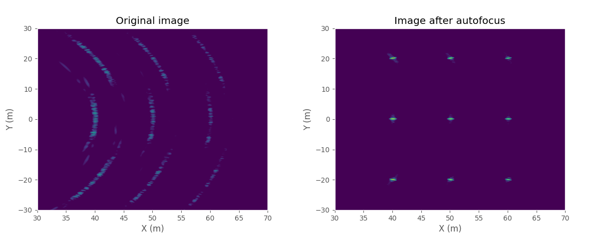
Image with position error (left) and the same image after applying the autofocus algorithm (right).

The maximum position error is 0.1 meters and it causes the image to be extremely defocused. Position error causes sidelobes to appear around each target.

The image was divided into nine subimages for autofocus so that each point target is in its own image. After applying six iterations of the autofocus algorithm the solved image looks almost exactly like the error-free ideal image.

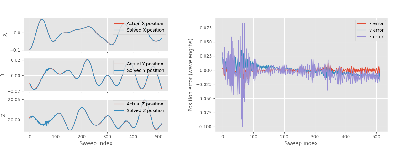
Solved 3D position error (left) and error in solved position in wavelengths (right).

The solved 3D position error matches well to the error that was added. The maximum error is 0.1 wavelengths in Z-direction and RMS error is 0.025 wavelengths. The image quality is the most sensitive to X-direction error that changes the measured distance the most, Z-axis error causes the smallest error in this case with low look angle as Z-axis is mostly perpendicular to the distance to the target.

Real data example

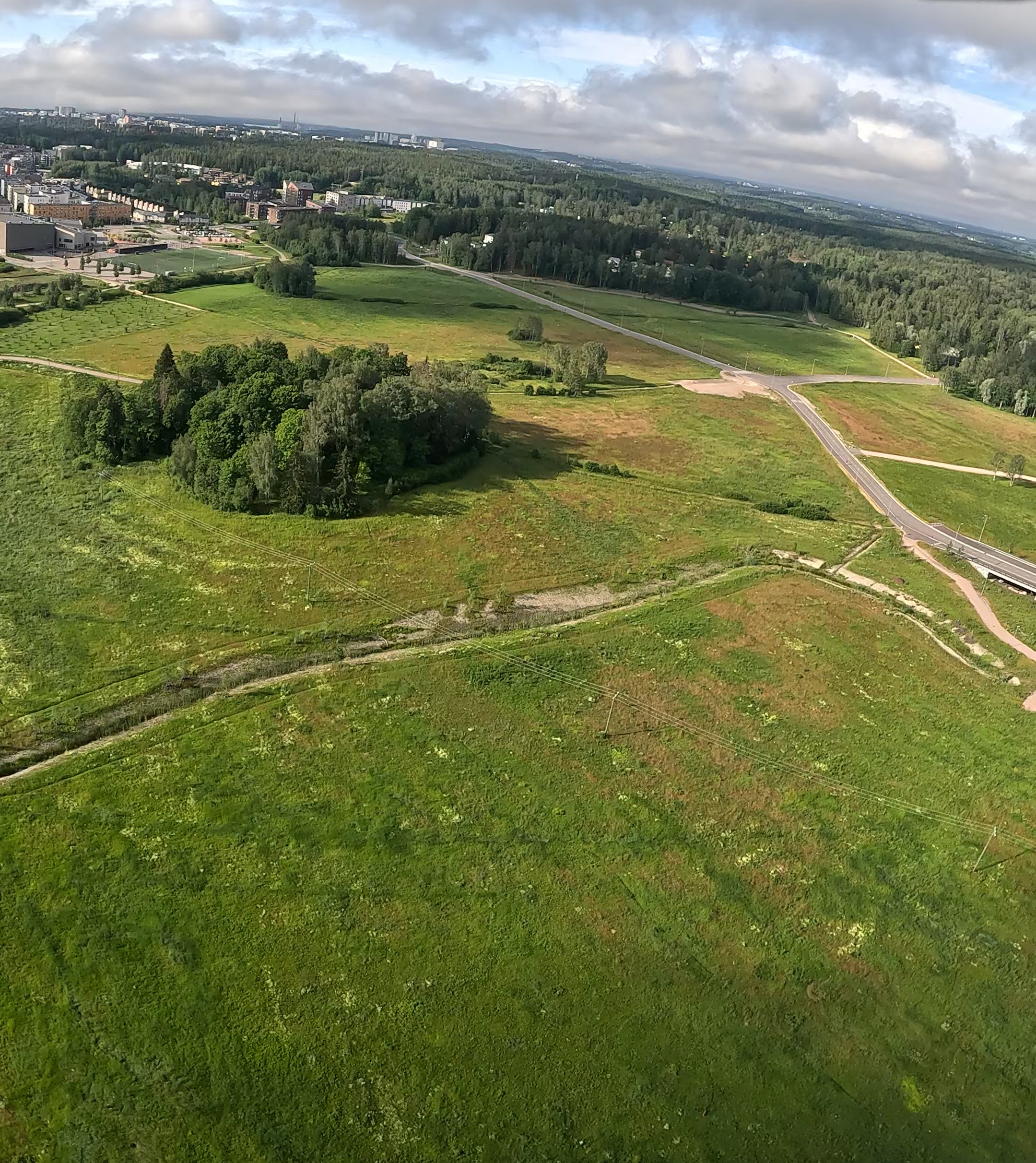
Camera image of the scene. This is from a different day and little farther away to capture more of the scene in the same image.

For a real data example I flew the radar drone in a straight line at 5 m/s velocity at 110 m altitude. The radar recorded full quad (HH, HV, VH, VV) polarizations with all four polarizations sampled at 1.8 ms repetition interval. The total number of samples is 20,000 for a total track length of 180 meters and 36 seconds of data capture time.

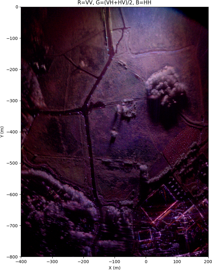
SAR image without autofocus using only the IMU and GPS for the radar position.

Without any autofocus algorithm and just relying on the GPS and IMU data fusion results in very poor quality image. The reported GPS position horizontal dilution of precision (HDOP) is on average 0.5 which is very good, but it's still not good enough for SAR accuracy requirement. RTK GPS would be much more accurate, but it requires a ground station and there isn't a small enough RTK GPS module that would fit well on the small FPV drone I'm using.

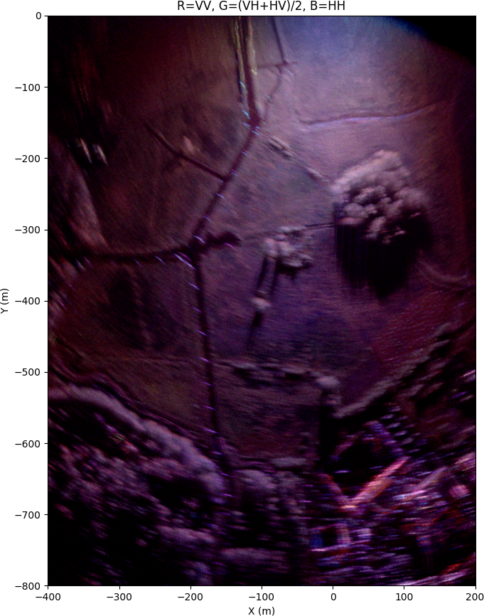
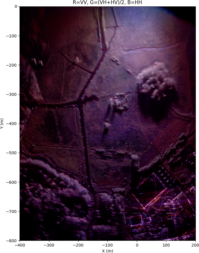
The same image after autofocus with GPGA 3D trajectory estimation.

After GPGA 3D trajectory deviation autofocus algorithm the image quality is much better. The image isn't still perfectly focused and it shouldn't be expected to, because no digital elevation model (DEM) is used. Instead every target is assumed to be on a flat plane at zero height. This assumption does not hold for a real scene as buildings and trees are at higher elevation than the ground and there is some elevation difference of the ground at different locations in the image.

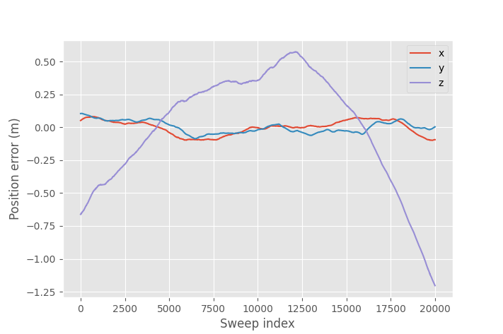
Solved position error.

The Z-axis solved position error is very large and it's unlikely that the real Z-axis error in the drone's flight elevation is this big and the error is likely due to the flat-plane assumption. If I disable Z-axis error estimation and force it to be zero the image quality is worse. For a better comparison here's a link to image with Z-axis correction for reference and also the image without autofocus.

The raw image dimensions are 6663 range samples by 13935 azimuth samples, requiring a total of $6663\times13935\times20000 = 1.9\times10^{12}$ backprojections to form the image when using ordinary backprojection. Using fast factorized backprojection image formation takes just 1.3 seconds on RTX 3090 Ti GPU, which is about 10 times faster than non-factorized backprojection. The final fully polarized image takes four times longer as it requires generating image for each of the four polarizations.

Autofocus uses a smaller image size of 2333 x 12541 pixels and divides it into 10x10 grid for a total of 100 subimages. Autofocus is only calculated for one polarization and the same solved position is used also for the other polarizations. The starting lowpass window size is 2000 samples and it's reduced by a factor of 0.7 every iteration until it's below 10 samples. The total number of iterations is 15 and the calculation takes a total of 17.5 seconds. It's a significant increase compared to the time it takes to form a single image due to requiring multiple image formations, but since the image formation is so fast when implemented on GPU it doesn't matter that much. Less iterations could work in this case, but in general these settings work well.

Antenna pattern normalization

Patch of ground illuminated by the radar. Three different areas for normalizing the reflectivity are colored.

The received power from a target depends on the target's distance to the radar, location in the antenna beam, and the radar reflectivity of the target. Radar reflectivity is what we want to determine and amplitude variations caused by the distance and antenna pattern is something that should be removed from the radar image.

Received power of a single radar pulse from a target can be written as:

$$P_r = C \frac{\sigma G_{rx}(\theta, \phi) G_{tx}(\theta, \phi)}{r^4}$$

$C$ is a constant that includes transmit power, receiver gain and other radar constant factors affecting the received power, $G_{rx}$ is the receiver antenna gain, $G_{tx}$ is the transmitting antenna gain, $r$ is the distance from radar to the target, and $\sigma$ is the radar reflectivity of the target.

Amplitude of the received signal is proportional to square root of $P_r$. It would be possible to add normalization in the backprojection calculation, but it's more efficient to calculate backprojection of the power received from a reference reflectivity separately:

$$P_{ref} = C \sum_{p \in \mathcal{P}} \sum_{n=1}^N \frac{\sigma_{ref} G_{rx}(\theta_n, \phi_n) G_{tx}(\theta_n, \phi_n)}{r^4}$$

$\mathcal{P}$ is the set of pixels in the image, $N$ is the number of radar measurements, $\theta_n$ and $\phi_n$ are elevation and azimuth angles to the pixel at $n$th position, and $\sigma_{ref}$ is the reference reflectivity where we want to normalize.

Removing the antenna pattern and distance variation from SAR image $I$ using $P_{ref}$ can be done by simply dividing the squared image by the reference power:

$$\sigma_0 = \frac{|I|^2}{P_{ref}}$$

$P_{ref}$ can be calculated on a coarser grid and number of sweeps can be decimated since antenna pattern doesn't change very fast making it faster to calculate than image backprojection.

We could simply set $\sigma_{ref} = 1$ and this is valid option if we want to normalize to point targets, but depending on how exactly the ground reflectivity is defined some other options are also available. Reflectivity of the ground can be defined in multiple ways. The most common one is to define $\sigma = \sigma_0 A_{\sigma}$, where $\sigma_0$ is the radar reflectivity of ground per unit area and $A_{\sigma} = \delta x \delta y$ is the area of the patch on the ground.

The size of the patch that needs to be considered is the pixel resolution in the SAR image. Radar measures radials distance, which means that $\delta_r$ is a constant that depends on the radar parameters. The angular resolution of the radar $\delta_\varphi$ is constant, so $\delta y = 2r\sin(\delta_\varphi/2)$. For SAR image with non-isotropic antenna the resolution isn't as good, but antenna weighting is already included in the calculation and we can use the resolution with isotropic antenna.

This means that to normalize to ground reflectivity $\sigma_0$ we should set:

$$\sigma_{ref} = A_{\sigma} = \delta_x \delta_y = \frac{\delta_r 2 r \sin(\delta_\varphi/2)}{\sin(\theta)} = C \frac{r}{\sin(\theta)}$$

Constant factor $C$ can be merged with the constant factor in the $P_{ref}$ calculation. To avoid dividing by zero at zero ground range we can limit the $\theta$ used in calculation to angular size of the first resolution cell: $\theta_{\text{max}} \approx \arcsin(z/(z+\delta r)) \approx \pi/2 - \sqrt{2\delta_r/z}$.

$\beta_0$ or $\gamma_0$ can be calculated the same way by changing the $\sigma_{ref}$ definition. $\beta_0$ doesn't include any correction for the grazing angle and $\sigma_0 = \beta_0 \sin\theta$. The third definition is to calculate $\gamma_0 = \sigma/A_\gamma = \beta_0 \tan \theta$. This normalizes for the area of the patch that the radar sees. If the ground reflectivity would be completely diffuse so that it reflects equally well in all directions, then the reflected power only depends on the area of the target that the radar sees and only this definition would result in no incidence angle variation in the image.

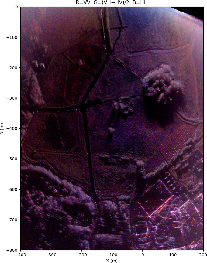
The previous measurement after removal of range and antenna pattern caused amplitude variation. The reflectivity is normalized to sigma zero.

After normalization the resulting image is much flatter in amplitude and at the edges where the signal-to-noise ratio is lower the noise floor is raised to visible level. Absolute radiometric calibration is not done since the constant $C$ has not been determined. It would require measuring a known reflectivity target and based on that measurement the $C$ constant can be determined. Incidence angle was calculates assuming a flat ground.

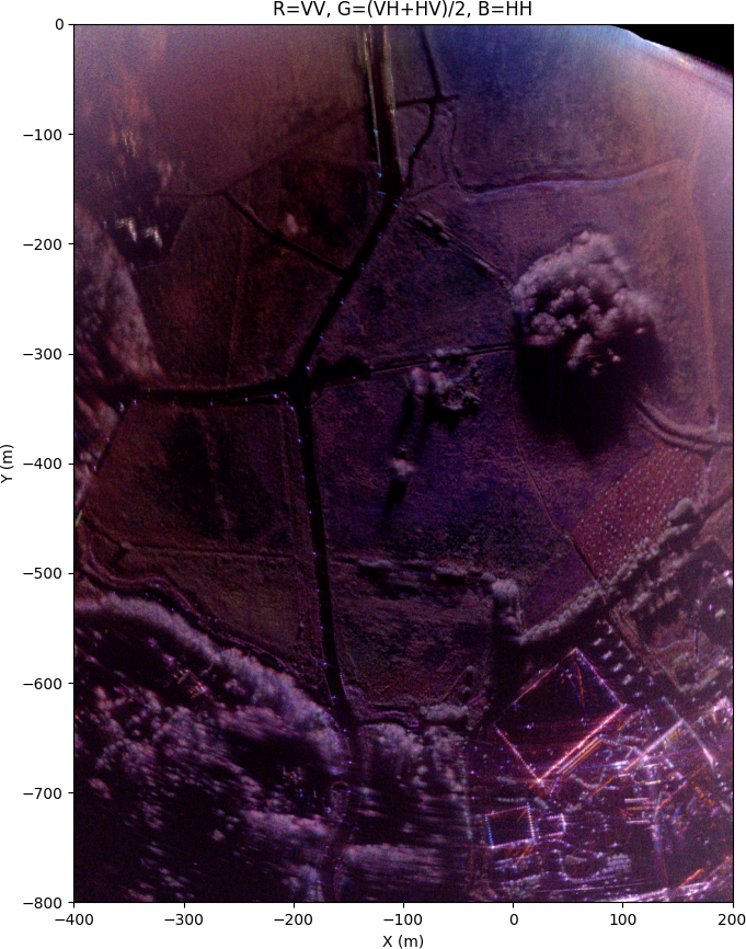
For comparison the same image with gamma zero is slightly brighter at farther distances where the grazing angle is low. Beta0 image looks very similar to the sigma0 image, there's only difference at extremely close ranges. Here's also a clickable link to sigma0 image. I recommend opening them in separate tabs for easier comparison.

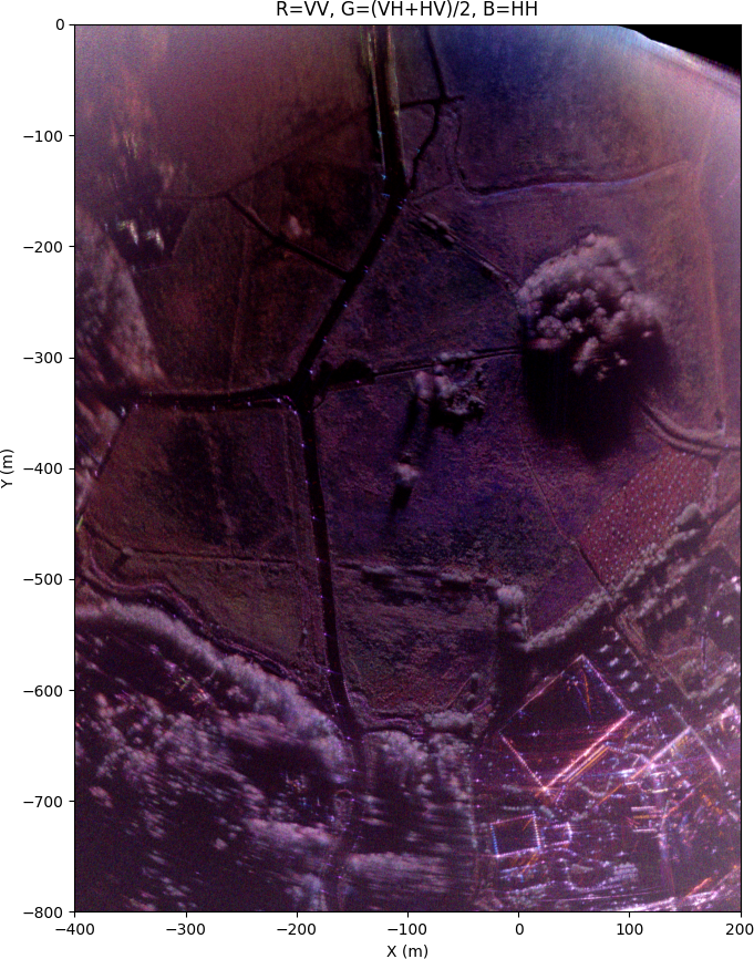
The first option of just setting $\sigma_{ref}=1$ results in very similar image to gamma zero normalization, only differing at very close distances. It turns out that at low grazing angle they are the same up to a constant.

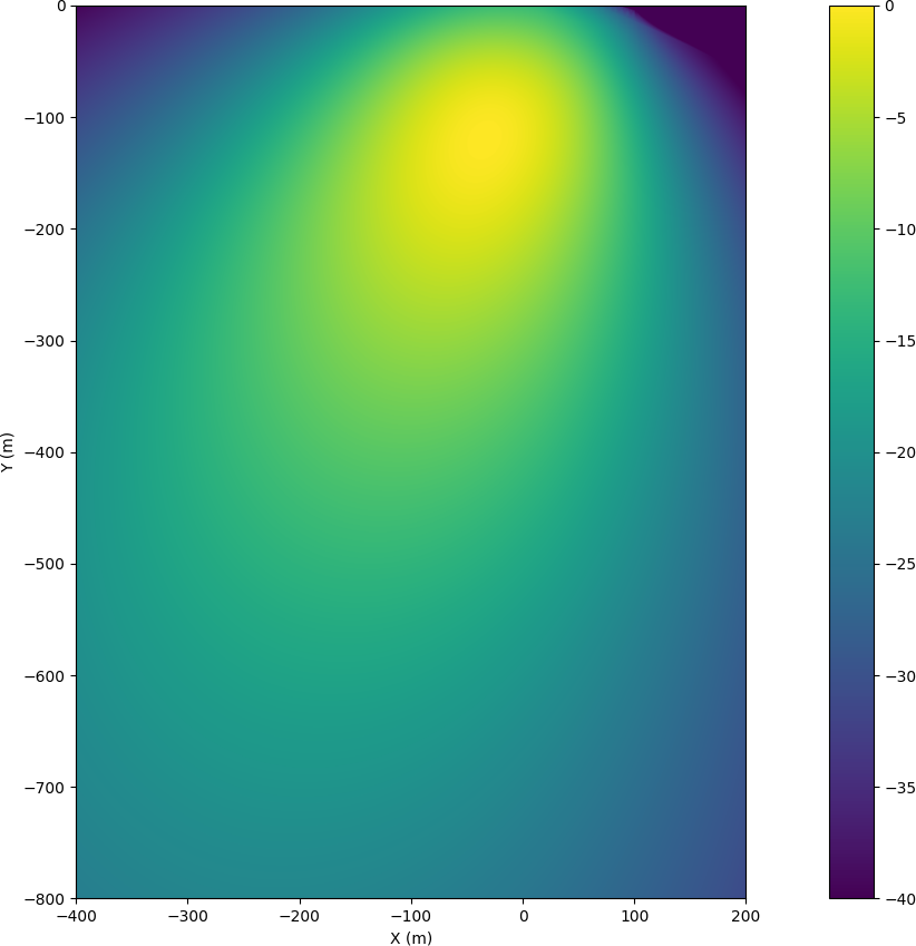
Visualized $P_{ref}$ for the previous image for VV polarization.

Plotting the image of $P_{ref}$ shows how the antenna illuminates the ground. The flight height was 110 m and the antenna was angled at 10 degrees below the horizon and the antenna boresight should hit the ground at 600 m distance. However, the best signal to noise ratio is obtained at 100 m since it's closer to the radar and antenna gain is still quite good at that angle.

Simulated antenna pattern was used in normalization and especially at far away angles from the boresight the actual radiation pattern can differ significantly. The uncertainty in antenna pattern causes amplitude difference at different angles, and in the polarimetric case the antenna pattern for H and V polarizations is slightly different which can cause errors in the relative channel amplitudes.

Polarimetric calibration

Block diagram of the radar with error sources affecting the measured polarization labeled.

A fully polarized radar measures four polarizations: HH, HV, VH, and VV. The first letter is the polarization of the transmitter, the second one is the polarization of the receiver, and V and H stand for vertical and horizontal. This is enough information to fully characterize the polarization response of a target and allows calculating received power for an arbitrarily polarized receiver antenna when the target is illuminated with an arbitrary polarization.

The transmission and reception of the different polarizations are implemented by a switch that selects which polarization is transmitted or received. The same electronics are used for all polarizations which results in good amplitude and phase match across all frequencies. However, due to polarization switches, slightly different lengths of SMA cables between switches and antennas, and small differences between the antennas, there are amplitude and phase differences between the polarizations. Additionally, the limited isolation of the switches and antennas causes some crosstalk between different polarizations.

To make accurate polarimetric measurements, channel amplitude and phase differences as well as crosstalk need to be measured and calibrated out. The effect of receiver and transmitter errors can be modeled as (Ainsworth, et. al):

$$\begin{bmatrix} O_{HH} & O_{HV}\\ O_{VH} & O_{VV}\end{bmatrix} = \begin{bmatrix} r_{HH} & r_{HV}\\ r_{VH} & r_{VV}\end{bmatrix} \begin{bmatrix} S_{HH} & S_{HV}\\ S_{VH} & S_{VV}\end{bmatrix} \begin{bmatrix} t_{HH} & t_{HV}\\ t_{VH} & t_{VV}\end{bmatrix}$$

$[O]$ is the observed polarization, $[S]$ is the true target scattering matrix, and $[t]$ and $[r]$ are matrices that model how the scattering matrix is transformed during the measurement by transmitter and receiver.

The previous equation can be written also in form:

$$ \begin{bmatrix}O_{HH}\\O_{HV}\\O_{VH}\\O_{VV}\end{bmatrix} = \mathbf{M} \begin{bmatrix}S_{HH}\\S_{HV}\\S_{VH}\\S_{VV}\end{bmatrix} $$

$\mathbf{M}$ is a 4x4 complex valued matrix that contains all the error terms that affect the target measurement.

A simple error correction method is to assume that there is no crosstalk and that absolute radiometric correction is already done. In which case $\mathbf{M}$ can be written as:

$$\mathbf{M} = \begin{bmatrix}k\alpha&0&0&0\\0&1/\alpha&0&0\\0&0&\alpha&0\\0&0&0&k^{-1}\alpha^{-1}\end{bmatrix}$$

$\alpha$ corrects for the imbalance of $HV$ and $VH$ measurements and $k\alpha$ corrects for $HH$ and $VV$ imbalance. Due to reciprocity, we should have $HV = VH$ and we can solve for $\alpha$ from the measured data by calculating the amplitude and phase difference between the measured $HV$ and $VH$ polarizations. Calculating the correlation matrix $C = E(O O^\dagger)$, where $E(\cdot)$ calculates the mean over all pixels in the SAR image and $\dagger$ is conjugate transpose, we can solve for $\alpha$:

$$\alpha = \left|\frac{C_{VHVH}}{C_{HVHV}}\right|^{1/4} \exp(j\text{Arg}(C_{VHHV})/2)$$

For example: $C_{VHHV} = E(O_{VH} O_{HV}^*)$. This calibration was already performed in the previous images so that the HV and VH channels could be summed for visualization (with $k=1$). Determining the $k$ factor is harder and requires measuring a target with a known scattering matrix, usually a corner reflector.

Scattering matrices of trihedral and dihedral corner reflectors at various angles. By measuring a known target, the polarimetric calibration matrix can be solved.

This simple measurement is enough to calibrate the biggest error sources, but for more accurate result the crosstalk terms should also be solved. There are several different polarimetric calibration methods and the one I decided to implement is "Orientation angle preserving a posteriori polarimetric SAR calibration" by T. L. Ainsworth, L. Ferro-Famil and Jong-Sen Lee. This method works by calculating correlation matrix from a SAR image of a scene, and only assuming scattering reciprocity (HV=VH) calculates most of the error terms based on the expected form of the correlation matrix. However, even with this method, at least one measurement of a known target is required to determine the $k$ calibration factor.

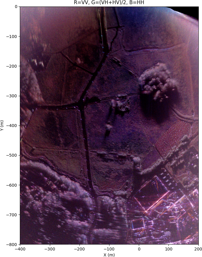
The previous image with polarimetric calibration.

After the polarimetric calibration, the largest difference is that the HH and VV channel amplitude balance was corrected increasing the VV channel power making the image redder compared to the uncorrected image.

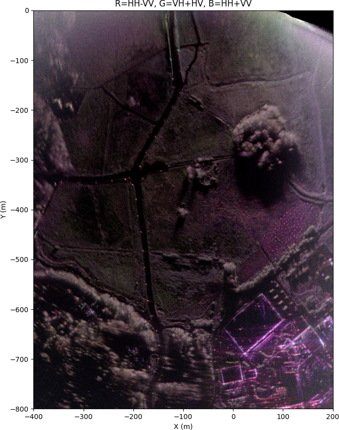
Pauli decomposition of the calibrated image.

After calibration, polarimetric decompositions, such as Pauli decomposition, can be applied. This is often used presentation for SAR data since it can be interpreted physically. The three channels are: HH+VV, which corresponds to targets where H and V polarization return at the same phase, for example a sphere or trihedral corner reflector. HH-VV corresponds to a dihedral reflector at 0 degrees, where one of the polarizations is flipped in phase. The last channel VH+HV corresponds to targets that return orthogonal polarization, such as 45 degree oriented dihedral reflector.

For surface targets, HH+VV corresponds to single or odd number of bounces, and HH-VV double or even number of bounces. Targets that depolarize the reflection, such as tree canopy are visible on the HV+VH channel.

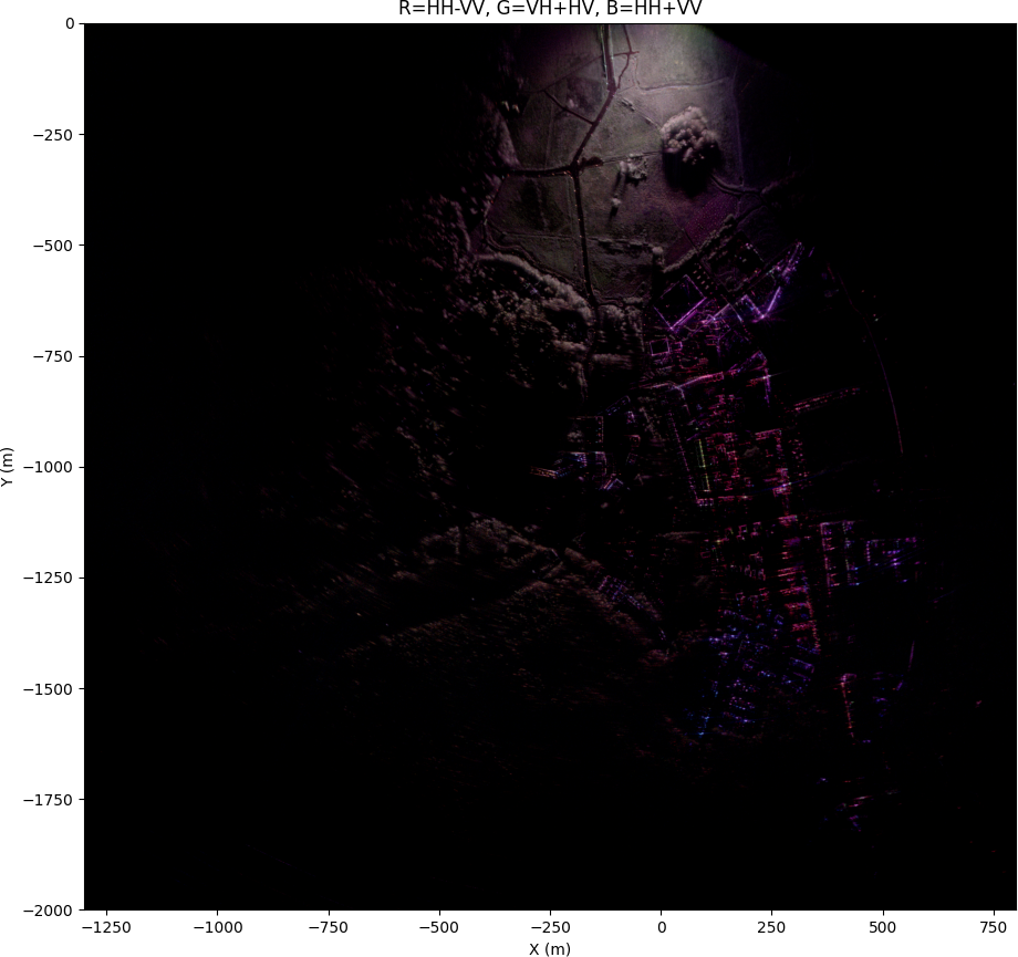
Full SAR image with Pauli decomposition and without antenna pattern normalization.

In the fully zoomed-out image, quite lot of details can be seen even at long distance, but the grazing angle at far away is very low, so only tree tops and buildings are visible and shadowing is severe. This is without antenna pattern normalization, since it doesn't make sense to normalize to flat ground that isn't visible at long range, but the polarimetric calibration is still applied.

Buildings at (+250 X, -1000 Y) with lot of sharp corners look very different from the surrounding trees and grass, which reflect a lot of cross-polarization. Using polarimetric image, it's possible to classify the target response, such as vegetation or artificial targets, which is one of the main uses of polarimetric SAR imaging.

VideoSAR

When a long radar measurement is divided into multiple short images, the result can be turned into a video. The drone flew autonomously a circular pattern over a field while the radar recorded continuously. Afterwards I autofocused and generated SAR images of short sections of the data, then synced them with the GoPro recording. The video is played back at 2x speed.

Each image has 2048 radar measurements, with 75% overlap between consecutive images. Having more data in each frame improves the image resolution and decrease the amount of noise, but lowers the frame rate in the video. The high overlap increases the frame rate as a new frame can be created when there is 25% of new data instead of waiting for a full window size and allows for good quality image with reasonable frame rate.

Each frame is autofocused individually and the solved position is used for the future frames. Apart from this, no inter-frame stabilization is performed. There are some small geometric errors, but overall the stability between frames is quite good. Antenna pattern is normalized to gamma0 and image edges with low SNR are cut out. Radial lines appear on some frames caused by RF interference.

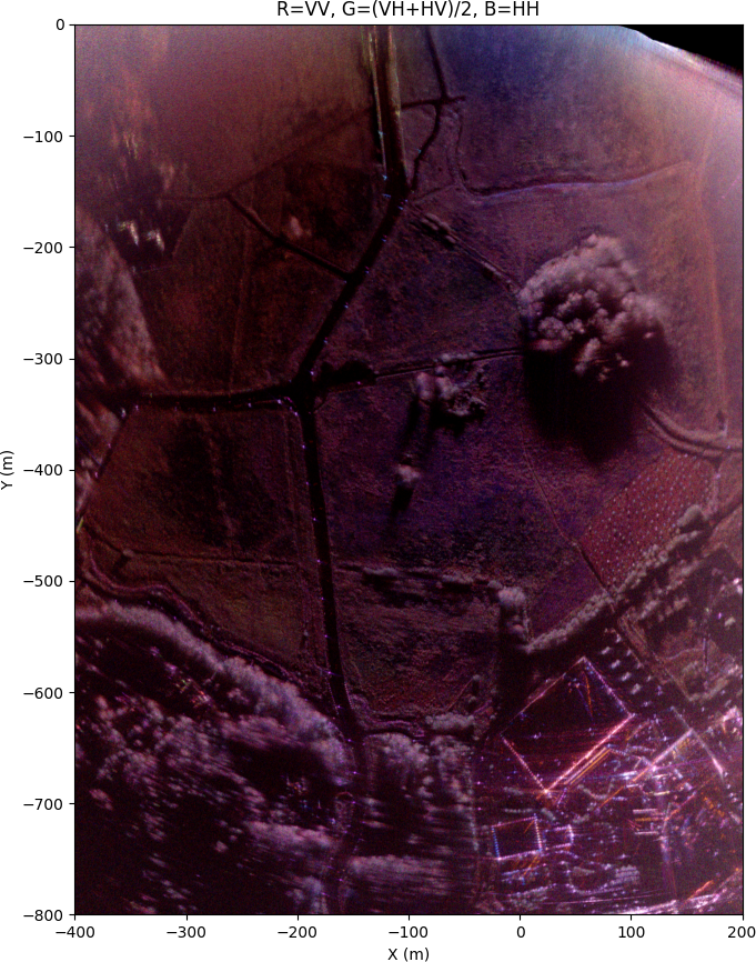
Urban scene

I captured another scene with more buildings. The drone flew in a straight line at height of 110 m and a speed of 5 m/s for 72 seconds, covering a total track length of 360 m. During this time the radar captured 40,000 sweeps.

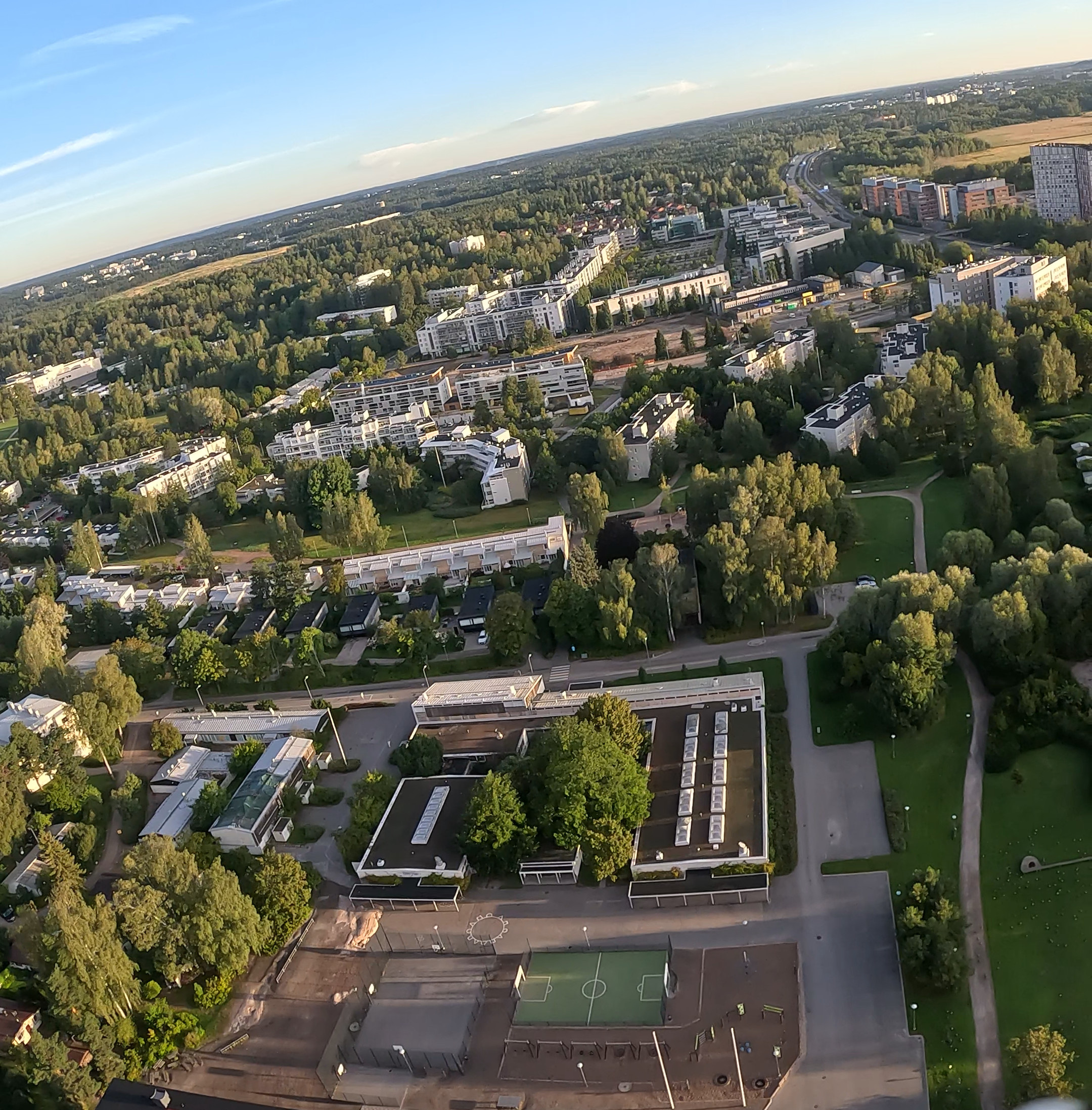
Camera image of the scene.

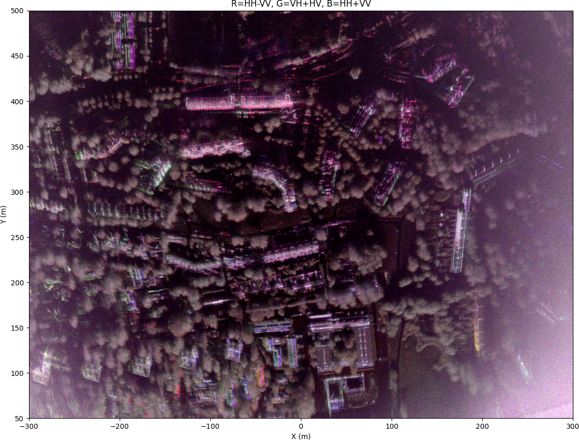
Image of urban scene after autofocus, antenna pattern normalization, polarimetric calibration, gamma zero normalization, and Pauli decomposition visualization. The camera image is taken from approximately X=100 m.

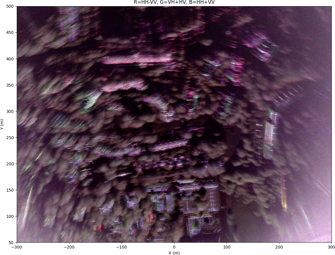
Autofocus required 41 seconds for this scene, and image formation took 2.3 seconds per polarization. The resulting image is 6663 by 27863 pixels. Autofocus improves the image quality significantly. Without autofocus the image is badly unfocused.

Conclusion

A complete software pipeline for autofocusing and calibrating polarimetric SAR image was presented. Autofocus algorithm that uses generalized phase gradient autofocus (GPGA) and 3D trajectory deviation estimation to solve for the 3D position error was introduced. Using GPU accelerated fast factorized backprojection even very large SAR images can be focused very quickly.

The resulting image quality is very good especially considering that this might be one of the cheapest drone mounted SAR systems.

The software is open sourced and available at: https://github.com/Ttl/torchbp.