Introduction
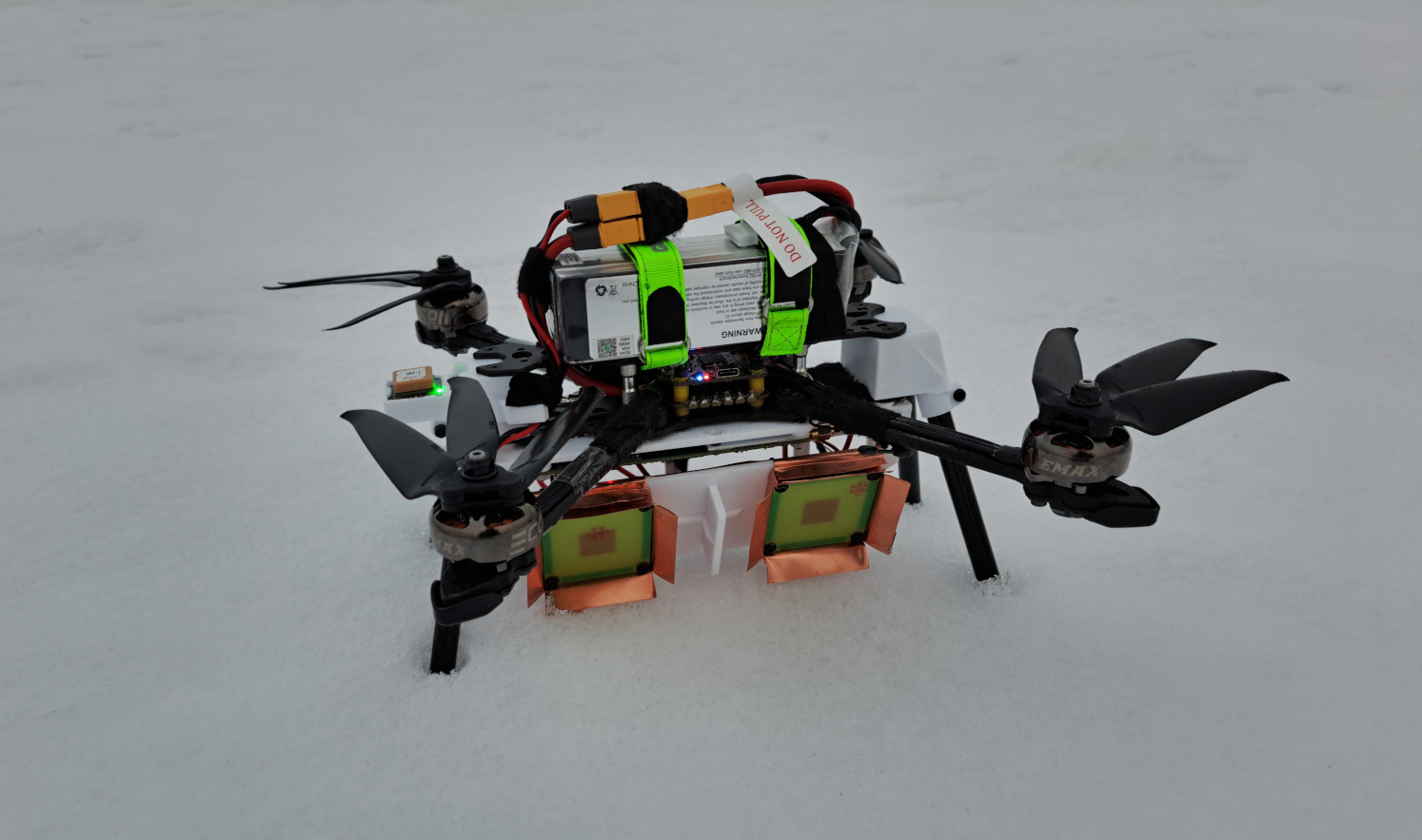
Radar drone ready to take off from snow.
I have made several homebuilt radars and done some synthetic aperture imaging
testing with them on the ground. I have wanted for a long time to put a radar on
a drone and capture synthetic aperture images from air. When I last looked at
this few years ago, medium sized drones with payload capability were
around 1,000 EUR and up. For example in Low-Cost, High-Resolution, Drone-Borne SAR
Imaging
paper by A. Bekar, M. Antoniou and C. J. Baker, the imaging results look
excellent. They used DJI S900 drone with a list price of about 1,000 EUR. The
price for the whole system is quoted to be £15,000, which is a way too
high for my personal budget even just for the price of the drone. Many other
papers use similar style medium sized drones designed for carrying cameras and
they are usually equipped with RTK-GPS for accurate positioning.
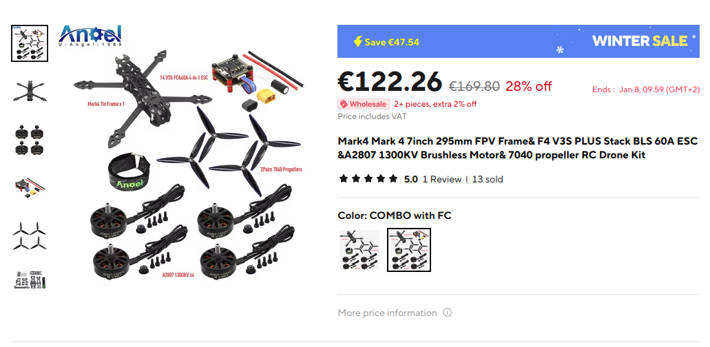
One of many cheap Chinese FPV kits.
Recently small FPV drone prices have dropped a lot. Small 5 and 7 inch propeller quadcopters can be bought for about 100 EUR from China (not including battery and RC controller). Despite their small size they are able to lift about 1 kg or even heavier payload which is plenty for a small radar.
I bought the cheapest Chinese no-name 7-inch FPV kit and a small GPS+compass module to support autonomous flying with the goal of making a light weight synthetic aperture radar system that it can carry.
Synthetic aperture imaging
A single-channel radar can only measure the distance to a target and is unable to detect the angle of the target. When multiple receiver channels are arranged in a line, the signal travels slightly different distances to each receiver based on the target's angle, causing phase shifts in the received signals. These phase shifts allows calculating the angle of the target.
Angular resolution (\(\Delta \theta\)) of antenna depends on its size approximately as: \(\Delta \theta \approx \lambda/D\), where \(\lambda\) is the wavelength, and \(D\) is the diameter of the antenna. For example to have 1 m resolution at 1 km distance requires 0.03° angular resolution with 6 GHz RF frequency. This would require antenna size to be about 100 meters.
Instead of making a single large antenna, it's possible to move a single radar and take multiple measurements at different positions. If the scene remains static, this approach yields the same results as having one many channel radar system with big antenna. With synthetic aperture radar it's possible to attach a single-channel radar to a drone, fly it while making measurements, creating a large synthetic aperture that provides exceptional angular resolution.
Radar design
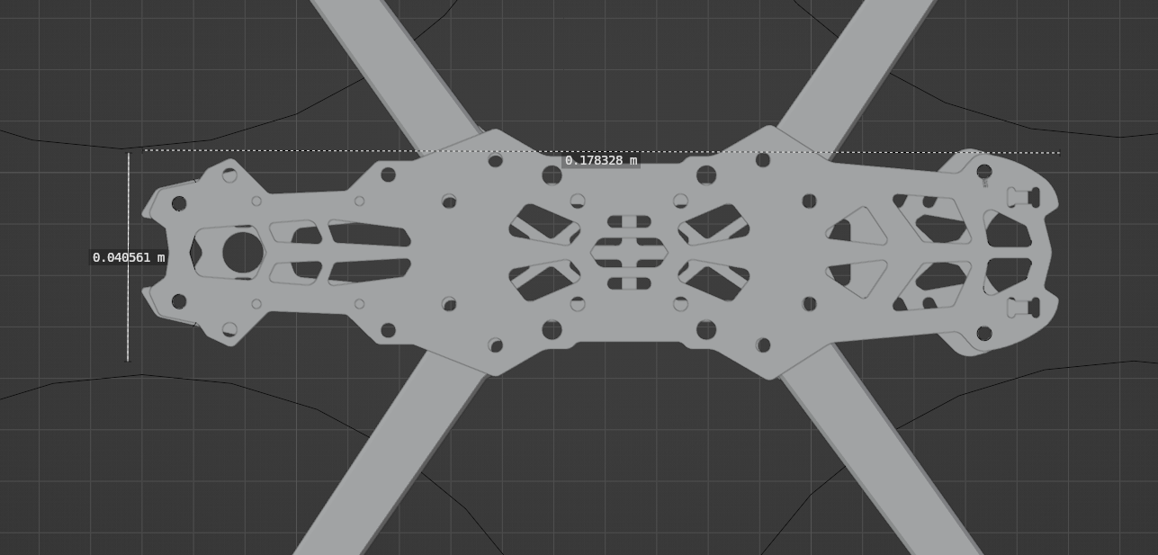
Dimensions of the drone frame. (3d model source)
The design goal for the radar is to get the best imaging performance while being able to fit into the FPV drone and achieving it with minimal budget (<500 EUR). The budget limitation rules out using any low-loss RF materials and both electronics and antennas should be implemented with lossy FR4 PCB material.
The drone is quite small and this limits the maximum size of the radar. The width of the frame is about 40 mm and propeller tip-to-tip distance is 50 mm across the frame. Length is about 170 mm, which is much more than width and means that ideally the radar is skinny. For example Raspberry Pi is 56 x 85 mm which is too wide. The small size severely limits on what the radar can include.

Block diagrams of FMCW (left) and pulse radar (right).
There are several possible architectures for the radar. I previously made pulse radar that is about 64 x 132 mm. That's little too wide for the drone, but I believe it would be possible to shrink it a little. Issue with that radar is that the maximum bandwidth is about 100 MHz and it's limited by the ADC sampling rate. This corresponds to a range resolution of 1.5 m, which isn't quite high enough for a detailed image. It's hard to get much larger ADC bandwidth on a reasonable budget and fitting high speed ADCs on the limited space is also an issue. There's also a variation of pulse radar that has two ramp generators, one for RX and one for TX. This results in low frequency IF signal like with FMCW radar. This is an architecture that is often used on SAR radars as it allows for high RF bandwidth without requiring high speed ADC.
Since pulse radar with switched antenna can't transmit and receive at the same time, pulsed radar maximum pulse length is limited by the time it takes for the pulse to travel to the target and back. With for example 100 m minimum distance, the maximum pulse length to not miss any part of the pulse is only 670 ns. Because pulse radar needs to divide measurement time between transmission and reception it reduces the average transmit power and decreases the signal-to-noise ratio. Large number of very short pulses also complicates the image formation. Time taken by the SAR image formation scales with the number of pulses and very short maximum pulse length requires transmitting very large number of them for a good SNR image.
FMCW radar can transmit and receive at the same time and which improves the signal-to-noise ratio. The maximum sweep length is only limited by the synthetic aperture sampling speed requirements but it can be hundreds of µs. Unlike pulse radar, there is also a minimum sweep length requirement, since reflected signal is mixed to the transmitted signal it needs to be received while the sweep is still being transmitted. Long sweep length allows collecting much more reflected power per one sweep. Pulse radar could also use separate TX and RX antennas so that this wouldn't be an issue, but that removes its advantages compared to cheaper to implement FMCW radar. Separate transmit and receive antennas require more space, but due to large maximum length it should be possible to fit two small antennas side-by-side under the drone.
In general FMCW radar has advantage for short range and slow moving platform applications. Pulse radar is required when long range (more than few km) is needed.
RF design

FMCW radar architecture.
Above is the block diagram of the RF parts of the FMCW radar with dual-polarized antennas. The sweep is generated by PLL, it's passed through a variable attenuator and then amplified by the power amplifier. Most of it is passed to the transmit antenna, polarization switch controls whether vertically or horizontally polarized antenna is used. Part of the transmitted signal is coupled to the receiver mixer, where it's mixed together with the received reflected signal that has been amplified by the LNA. Receiver also has a polarization switch, together with the transmit switch it allows the radar to receiver and transmit any of the four combinations of polarizations. The mixer outputs a low frequency signal that is amplified and then digitized by the ADC. Some filtering is needed in the receiver to avoid large out of band signals and ADC aliasing.
DAC or DDS based sweep generation would likely be better than PLL. DDS phase noise is often better and it can change frequencies essentially instantly compared to PLL, but PLL is chosen because it's cheaper and requires less space.
RF frequency is going to be around 6 GHz as this is the maximum frequency where there are many cheap RF components for consumer applications. The highest output power cheap power amplifiers at this frequency output around 30 dBm. Low noise amplifiers for the receiver with 1 - 2 dB noise figure can also be obtained cheaply.
Receiver is direct conversion architecture and the mixer does not have any image rejection. This causes both frequencies above and below the transmitted signal to be converted to the same output frequency. This is not ideal as noise below and above the instantaneous sweep frequency is received increasing the noise floor by 3 dB. IQ sampling receiver that could reject the other sideband would need two mixers and ADCs. For only 3 dB increase in the signal to noise ratio, I didn't think it was worth the cost and PCB space.
Polarization switches allow choosing which polarization is used to transmit and receive. H is horizontal and V is vertical polarization. This allows measuring four polarizations: HH, HV, VH and VV, where the first letter denotes TX polarization and the second RX. Some targets reflect some polarizations more than others and it is used in remote sensing to determine properties of reflected targets. For example many smooth targets often reflect the same polarization with shape of the target determining if it reflects more HH or VV components. Forest and vegetation usually has higher cross-polarized HV and VH component reflection compared to roads and bare ground due to multiple reflections inside the vegetation.
Although H and V antennas are drawn separately in the block diagram, this doesn't mean that the system requires four antennas. It's possible to design antenna with two ports, one which radiates H and the other V polarization. Dual polarized antenna doesn't necessarily need any more space than single polarized antenna.
It would be possible to receive both H and V at the same time if the radar would have two receivers. This would have some advantages, it would allow removing the RX polarization switch which would decrease the losses and only the TX should be switched allowing more time for each measurement which would also increase SNR. It would also allow transmitting sweeps faster as there isn't need to multiplex the receiver polarization switch. However, I didn't consider it being worth the cost.
TX-RX leakage

TX-RX leakage can saturate the receiver on high powered FMCW radar if the leakage is too high.
More RF power generally improves the signal-to-noise ratio, but since FMCW radar transmits and receives at the same time, it's important to consider the TX-RX leakage signal. The receiver must be sensitive enough to be able to detect the thermal noise floor at -174 dBm/Hz without saturating due to leaked RF power from the transmitter antenna. Typical maximum input power that saturates the LNA is around -20 dBm. With +30 dBm transmitted power more than 50 dB isolation is needed between transmitter and receiver to prevent the receiver saturation. Even more isolation might be required if some other receiver component, such as ADC, saturates first. The variable attenuator before PA can be used to decrease the transmit power in case high enough isolation antennas don't fit in the drone. It also affects the receiver mixer's LO power, but mixers LO input power range should be large enough for it to not be an issue.
Link budget
The equation for the received power at the receiver input can be written as:
where \(P_t\) is the transmitter power, \(G\) is the antenna gain, \(\lambda\) is wavelength, \(\sigma\) is radar cross section of the target, and \(r\) is range to the target. This is the received power from one pulse. Synthetic aperture is formed by sending multiple pulses while moving and these can all be coherently summed together to increase the signal to noise ratio. If image is formed from \(n\) pulses, the received power can be multiplied by \(n\) to get the received power in the whole image.

Radar measures radial distance δr, which is different from the ground resolution δx. δp is length of the area perpendicular to the antenna beam.
For a patch of ground, the reflectivity can be defined as: \(\sigma = \sigma_0 A\), where \(\sigma_0\) is reflectivity per unit area and \(A = \delta x \delta y\) is the area of the ground patch. \(\delta x\) is the resolution in the X-direction and \(\delta y\) is resolution in cross-range direction. The radar measures radial distance \(\delta r = \delta x \cos \alpha\), which causes the ground resolution to depend on the grazing angle \(\alpha = \sin{h/r}\), with \(h\) being the radar's height above the ground.
In this case \(\delta x \approx \delta y \approx 0.3 m\), depending on the radar parameters, range, and imaging geometry. Reflectivity of the ground patch depends on the material of the ground patch and the angle of illumination. Reflectivity of ground is generally higher when it's illuminated at 90 degree angle (in direction of the ground normal vector). This causes the specular reflection to reflect back to the radar. At smaller angles there is still some reflection back to the radar, but it decreases as the incidence angle decreases. Typical ground reflectivity is around -20 to 0 dBsm (decibels square meter) with moderate look angle. At very low incidence angle there is additional problems with shadowing as there won't be any return from a target that radar doesn't have an unobstructed line of sight.
The minimum detectable power is limited by thermal noise of the receiver. It can be written as \(kTBF\), where \(k\) is Boltzmann constant, \(T\) is receiver temperature, \(B\) is the noise bandwidth and \(F\) is noise figure of the receiver. It's a common mistake to confuse the noise bandwidth \(B\) with RF bandwidth, but they are not related to each other. Noise bandwidth is the minimum bandwidth where receiver can separate noise and signal from each other. By taking Fourier transform of the input signal, we can discard all the frequency bins that are beyond the signal we are currently looking at, and noise at those discarded frequencies won't affect the detection capabilities of the receiver. FFT resolution resolution is equal to \(1/t_s\), where \(t_s\) is the sweep length.
Setting the received power \(P_r\) equal to noise power and solving for \(\sigma_0\) we get noise equivalent sigma zero (NESZ) that is value often used for comparing synthetic aperture radars.
The number of pulses in image \(n\) could also be written as \(t_m \text{PRF}\), where \(t_m\) is the measurement time and \(\text{PRF}\) is pulse repetition frequency. Or equivalently \(l_m \text{PRF} / v\), where \(l_m\) is the length of the flown track, and \(v\) is the velocity of the drone during measurement. If the antenna points at a constant angle during measurement (stripmap image) the number of pulses in the image depends on the time that ground patch is illuminated by the antenna beam and can be much smaller than the previous number if the antenna beam is narrow. Quadcopter can easily fly pointing in arbitrary angle and it's possible to constantly point the antenna at the target (spotlight imaging) and this limitation doesn't necessarily apply in this case.
| Variable | Explanation | Value |
|---|---|---|
| \(P_t\) | Transmitted power | 30 dBm |
| \(G\) | Antenna gain | 10 dBi |
| \(\lambda\) | Wavelength | 5.2 cm |
| \(\delta x \delta y\) | Image pixel resolution | 0.3 x 0.3 m |
| \(T\) | Receiver temperature | 290 K |
| \(t_s\) | Pulse length | 200 µs |
| \(n\) | Number of pulses in image | 10000 |
| \(F\) | Receiver noise figure | 6 dB |
| \(\alpha\) | Grazing angle | 30 deg |

Noise equivalent sigma zero vs range with above listed parameters.
Plotting the NESZ as a function of range gives the above plot. There are some parameters that can be adjusted, mainly sweep length and the number of sweeps in image to slightly improve this figure. The requires NESZ for good quality image depends on the actual reflectivity of the ground, but typically for satellite based SAR NESZ is around -20 dBsm. With these parameters we should expect to see to around 1 - 2 km with ok image quality. This is slightly optimistic for drone SAR since 30 degree grazing angle at 2 km distance would require flying at 1 km altitude, which is much higher than is practical.
Pulse repetition frequency

Minimum alias-free pulse repetition frequency with 6 GHz RF frequency and with different number of time-multiplexed channels.
Radar image formation relies on the phase information of the received signal. If we consider a target that is 90 degrees from the antenna beam center (in the direction of movement) to avoid phase ambiguity, the maximum phase difference between two adjacent measurements needs to be less than 180 degrees. If the movement is larger than this, there can be multiple targets at different azimuth angles that have the same phase difference between measurements causing them to overlap in the image. Since both transmitter and receiver antennas move, a distance of a quarter wavelength between two measurements of the same target results in a half-wavelength difference in the distance traveled by the signal and a half-wavelength distance difference corresponds to 180-degree phase difference. At this spacing, targets at ±90 degrees will have the same 180-degree phase difference between measurements. If the measurement spacing is increased further more of the image starts to alias.
If the antenna is very directive then it's possible to use larger measurement spacing. Directive antenna won't radiate to large angles that would alias, and the more directive the antenna is, the larger the measurement spacing can be. However, since the drone is space-limited and antenna directivity is related to its size, it might not be possible to design a very directive antenna causing the maximum measurement spacing to be around quarter wavelength.
The common flying speed for a quadcopter is around 10 m/s, but flying speed can easily be decreased if needed. With 6 GHz RF frequency, the quarter wavelength is 12.5 mm (0.5 inches) and 10 m/s flying speed means that pulse repetition frequency needs to be at least 800 Hz. Since we have time multiplexed four different polarizations, we need to be able to measure all of them in this time.
PRF sets the requirement for maximum sweep length. With 4 * 800 Hz = 3.2 kHz PRF requirement this leaves maximum of 312.5 µs per sweep. However, some time needs to be reserved for time between sweeps due to limited locking time of the PLL. The locking time of the PLL is around 20 - 30 µs, leaving 280 µs for the maximum sweep length.
Required ADC sampling frequency
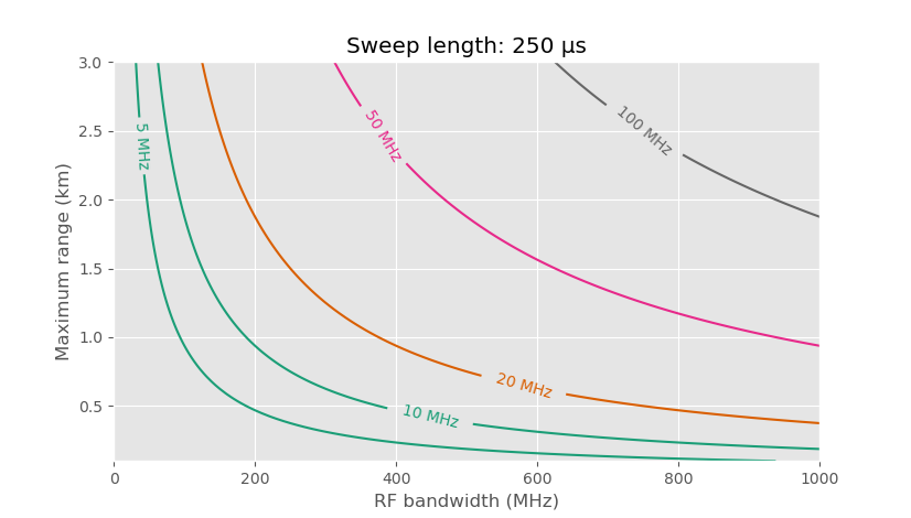
Required ADC sampling rate vs maximum range and RF bandwidth for FMCW radar with 250 µs sweep length.
FMCW radar mixes the received signal with a copy of the transmitted sweep, resulting in a sine wave signal at the mixer output with frequency depending on the range to the target. If the target is at distance \(r\), the IF frequency \(f\) can be calculated as: \(f = \frac{2 B r}{c t_s}\), where \(B\) is the bandwidth of the RF sweep, \(c\) is the speed of light, and \(t_s\) is the sweep length. The range resolution depends on the RF bandwidth \(B\) as \(\Delta r = \frac{c}{2B}\). For example, 150 MHz bandwidth is required for 1 m resolution, and 300 MHz bandwidth results in 0.5 m resolution.
If we have 300 MHz of RF bandwidth (0.5 m range resolution) and \(t_s\) is 280 µs as calculated earlier, then we can calculate the required ADC sampling speed given the maximum target range we want to detect. For example, with 2 km maximum range, the IF signal frequency is 14 MHz. The ADC sampling frequency needs to be at least double this due to Nyquist sampling requirement, and some additional margin is needed for the anti-alias filter roll-off. This results in a minimum ADC sampling frequency of about 35 MHz. I chose to use 50 MHz sampling frequency.
FPGA

Block diagram of digital parts.
The amount of data and strict timing requirements of the sweep generation make it difficult to handle with microcontroller and FPGA is necessary. Microcontroller is useful for more complicated tasks such as communication with the drone flight controller and ground station, configuring the radar, and writing the data to a filesystem. I decided to use Zynq 7020 FPGA, the same one I used in my previous pulse radar. It has FPGA fabric and a dual-core ARM processor in the same package. This FPGA is nominally 150 EUR from ordinary distributors, but is available for fraction of that from Chinese distributors.
The drawback of this FPGA is that the microcontroller doesn't have many high speed connections. For example SD-card and EMMC interfaces are limited to 25 MB/s, which is below the data rate of the ADC. It does have 1 Gbps Ethernet, but using that would require adding a Raspberry Pi or similar computer, which isn't possible due to size constraints. For instance, newer Ultrascale+ FPGAs support SD-cards with 52 MB/s and EMMC at 200 MB/s speeds, but they cost around 500 EUR and are not available from Chinese low cost distributors.
Zynq can have external DDR3 DRAM, but due to space limitations, it's not possible to fit enough DRAM to store the whole measurement in memory. With limitation of only one DDR3 module, the memory is limited to 1 GB, while size of the measurement can be several gigabytes.
This leaves only the option of implementing fast enough external communication interface in the programmable logic side of the FPGA. Luckily Dan Gisselquist (ZipCPU) has made GPL3-licensed SD-card and EMMC controller that supports faster high-speed communication modes than the hard IP included with the ARM processor.
At the time, sdspi controller hadn't been tested with real hardware at the speeds I required. To make sure I have something working if I'm unable to get the sdspi core working I connected the SD-card to the ARM processor's integrated controller, which is limited to 25 MB/s, and EMMC memory to the programmable logic side that is used with the sdspi controller. This way I'm able to at least use the SD-card with the integrated controller if the sdspi core isn't suitable, but this turned out to be unnecessary and the sdspi controller worked fine. In future versions, it would be better to also connect the SD-card to PL side using sdspi core for faster SD-card speeds.
I also added FT600 USB3 bridge IC that can be used to connect FPGA to PC. This is not needed for drone usage, but allows real-time connection to PC for other applications.

FPGA program block diagram.
FPGA functionality is quite simple at the block diagram level. The design primarily consists of a few independent blocks wired with either DMA or AXI bus to the processor. For radar operation, the radar timer block is important as it switches internal and external signals during the measurement. It needs to be implemented in the FPGA fabric to ensure that the timing is clock cycle accurate to achieve phase-stable radar measurements. AXI bus is memory-mapped on the processor side, allowing the radar to be controlled by writing values to fixed memory addresses.
A decimating FIR filter after ADC data input can be used to change the sample rate of the ADC data. It can decimate by 1, 2, or 4. For long-range measurements, the decimation should be disabled for the maximum IF bandwidth. But for shorter-range measurements it makes sense to use higher decimation value to decrease the amount of data that needs to be stored.
PCB
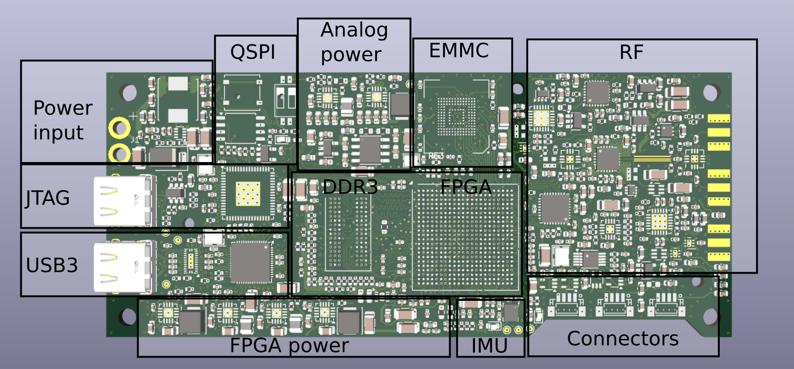
Labeled PCB 3D model in KiCad. Some 3D models are missing.
The PCB has six layers and is designed to be as compact as possible, with components placed closely together to minimize size. Since one-sided assembly is cheaper than assembling both sides, the bottom side is empty except for one SD-card connector that I will solder myself.
As with many of my previous radars, the RF part is a relatively small part of the PCB and the overall design effort. Digital electronics and voltage regulators take up the majority of the PCB space.
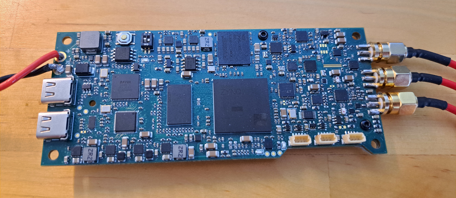
Assembled PCB.
The radar is designed to accept input voltage from 12 to 30 V and connect directly to the drone's battery eliminating the need for an external DC/DC regulator.
Due to space constraints, there wasn't enough space to fit four SMA connectors and I didn't want to use any miniature RF connectors. The top two connectors are switchable TX outputs for H and V polarization antenna inputs, while the bottom third one is RX input. The RX polarization switch is located on an external PCB and connects to one of the three four-pin JST connectors on the bottom right of the PCB. Another JST connectors is for flight controller's serial port, and the third connector is currently unused, but it could be used to connect for example GPS.
There are two USB-C connectors: one for JTAG programming and debugging of the FPGA, and the other connects to USB3 to FIFO bridge chip that enables fast data transfer to PC. It isn't needed in drone use, but it's useful for testing and other applications.
PCB dimensions are 113 x 48 mm. Width is just skinny enough to fit on the drone, while it could have been slightly longer.

This component is not sale for individuals.
After ordering the PCB I made an order for the components from Mouser. The order seemed to succeed fine and they accepted my money but I got the above email afterwards telling me that they can't sell me one of the components. Reason seems to be that the supplier of the component has forbidden them for selling it to individuals. This was very frustrating as there was absolutely no warnings on the website and I had already ordered the PCBs. I was unable to order this component from anywhere, but I did find older obsolete PE43204 pin compatible IC from obsolete component reseller. It's specified only for maximum of 4 GHz when the original was up to 6 GHz but it does seems to have low enough loss at 6 GHz to not cause too large issues.
After asking on reddit the reason is probably that the manufacturer of the component wants to know who they are selling to, to avoid their components ending up in defense applications. That's fine, but it would have been nice to know that in advance.
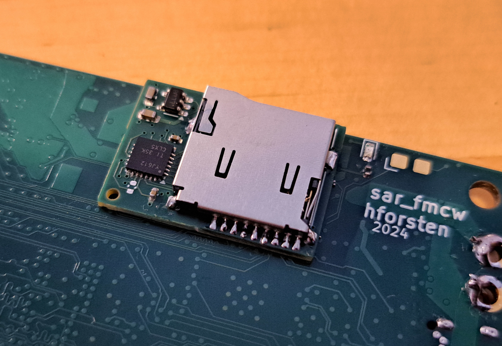
SD-card interposer PCB.
I did make one mistake: SD-card pins are connected to 1.8 V I/O pins, while they should be connected to 3.3 V I/O and SD-card didn't work with this lower voltage. The radar could be used without SD-card by storing the data into EMMC instead and then reading it through USB, but SD-card would be much easier to use. I really didn't want to order another PCB to just fix this one mistake and I managed to fix it by designing a small interposer PCB with level shifter that I soldered on top of the previous SD-card footprint. I wrote about it in more detail in a previous post.
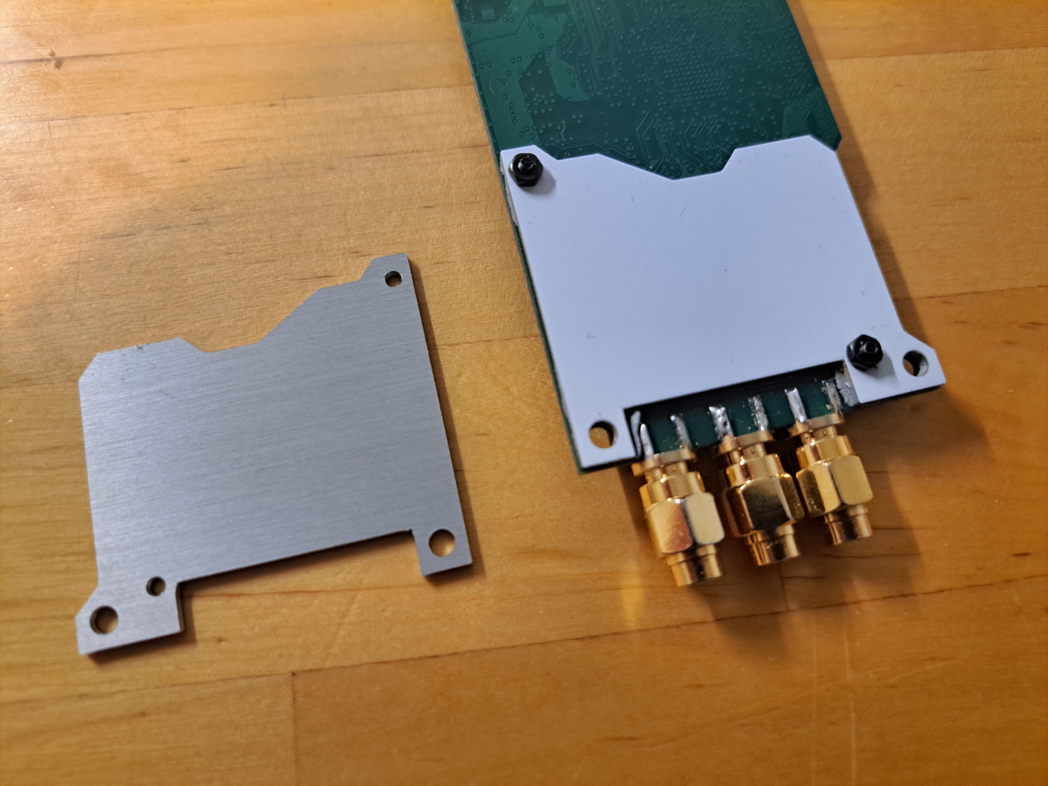
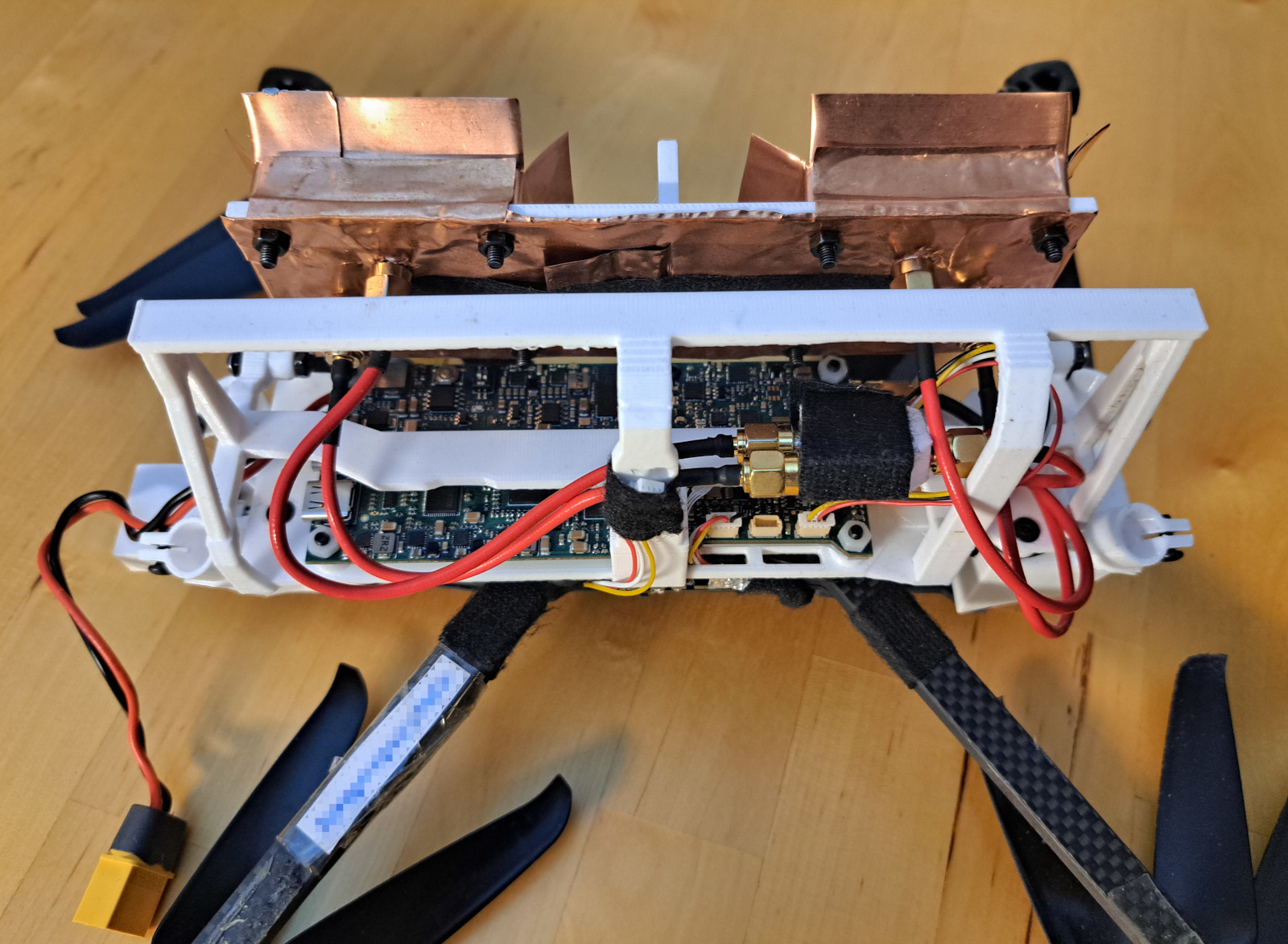
Aluminium PCB heatsink under the radar PCB.
Power amplifier can get quite hot if the transmit duty cycle is high. To keep it cool I ordered custom aluminium substrate PCB that I bolted under the radar PCB. Solder mask is removed under the PA and thermal pad is placed between the PCB and heatsink. This cost only $4 for 5 pieces and works very well.
Drone electronics
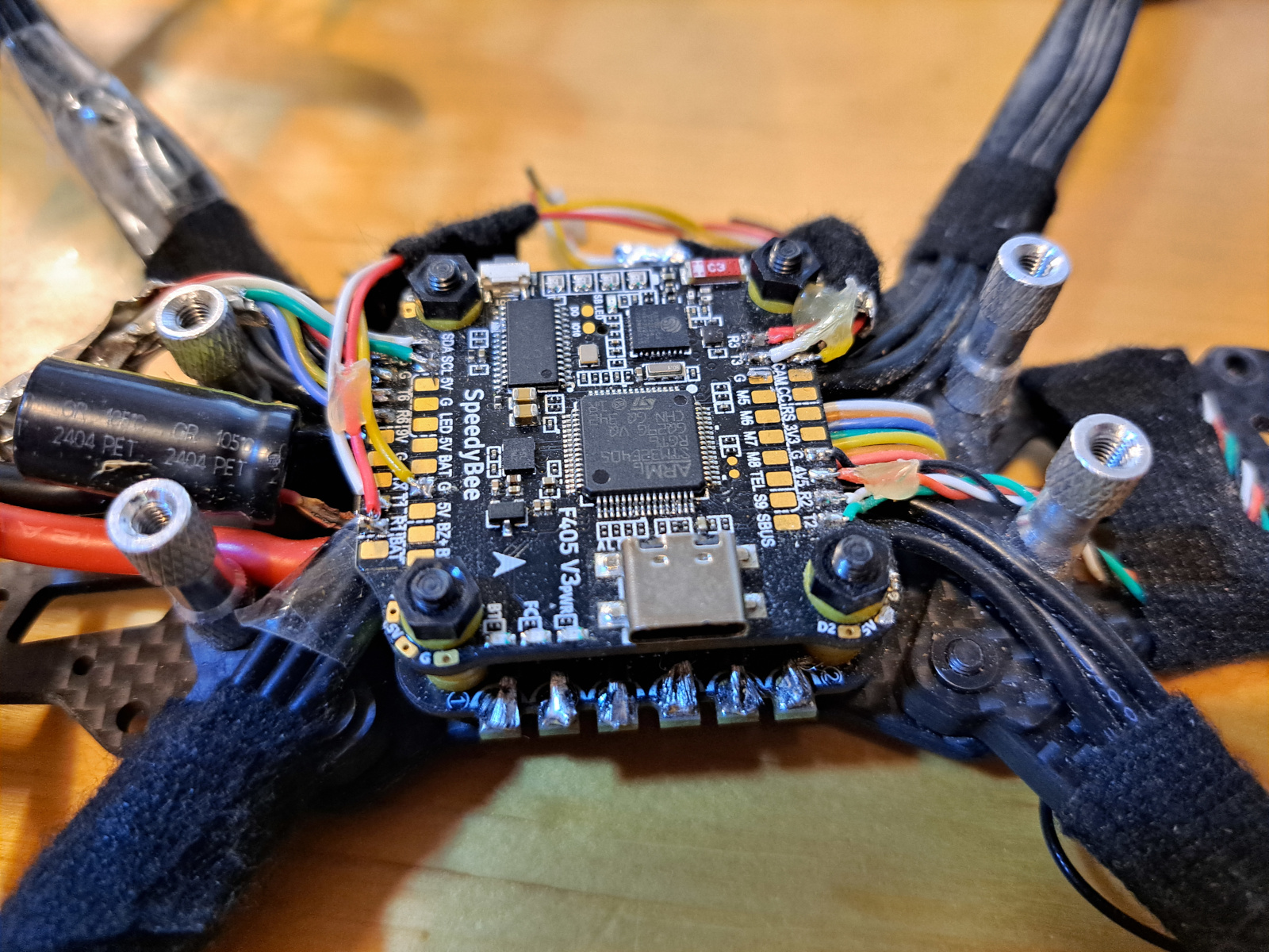
Speedybee F405 V3 flight controller.
Flight controller came with the drone kit. The included flight controller is Speedybee F405 V3. This is a cheap low-end flight controller with 1 MB of flash. It does the job, but I would recommend getting a little bit better flight controller with 2 MB of flash, the price difference isn't very large.
There are several possible flight controller softwares. The three most used for FPV drones are: Betaflight, Inav, and ArduPilot. The main differences of them are: Betaflight focuses on fast-response manual flying and doesn't have autonomous flight support, Inav shares lot of code with Betaflight and it includes some autonomous flight support, and ArduPilot has the most advanced autonomous flight capability with lot of features but it's more challenging to configure.
I chose to use Ardupilot and found it to be excellent for this purpose. It has very good IMU and GPS sensor fusion algorithm that is very helpful for improving the position accuracy. The flight controller can communicate with the radar through a serial port allowing it to enable and disable the radar during autonomous mission and provide position information for the radar.
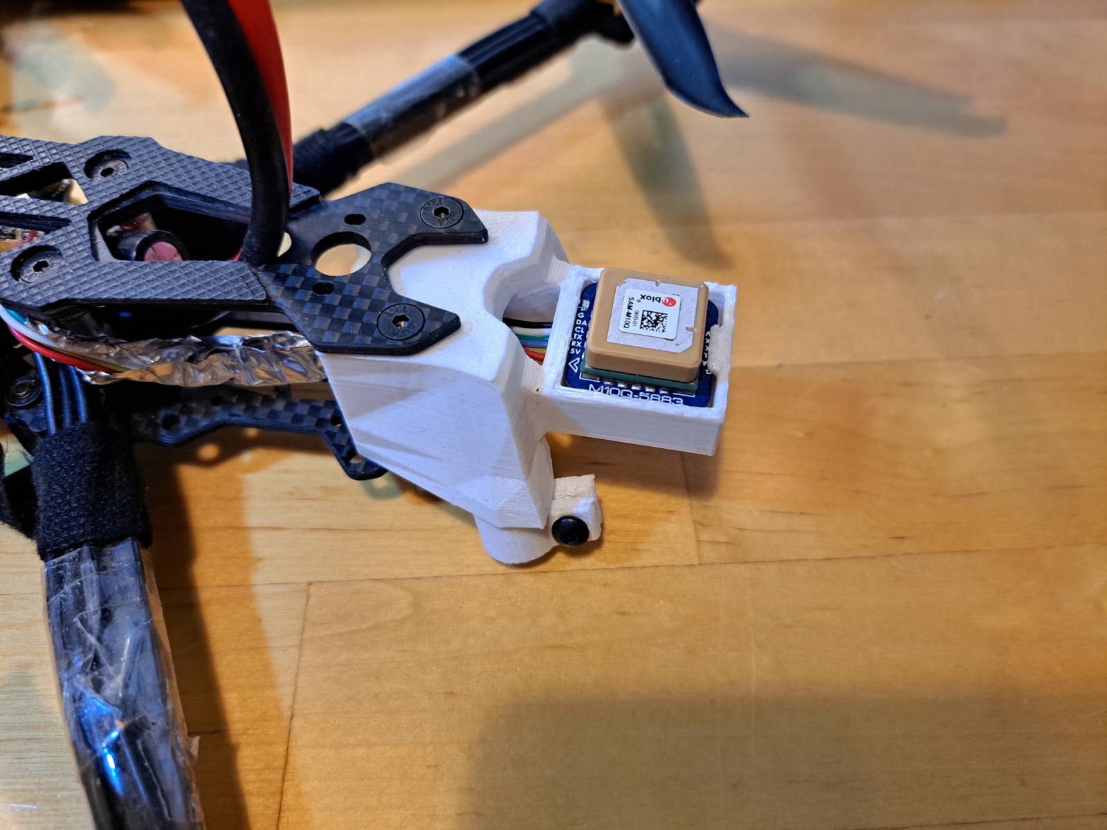
GPS with integrated compass. It needs to be mounted far away from the battery leads to avoid magnetic fields causing issues with the compass.
SAR imaging needs very accurate position information for proper image focusing. Position information should be accurate within to a fraction of wavelength, this is just few cm (1 - 2 inches) at this frequency. Many commercial SAR imaging drones use RTK GPS with a second stationary GPS receiver on the ground it's possible to obtain about 1 cm accurate positioning. The drawback is that it's much more costly than regular GPS and RTK GPS receivers are usually much larger than ordinary GPS receivers which makes it very difficult to fit it in this drone.
Good non-RTK GPS might be accurate to about 1 m accuracy. This large positioning errors cause significant errors in the image if not corrected. Luckily, it's possible to solve for position error from the radar data which is called autofocusing. With drawback of needing more processing during the image formation for autofocusing, it's possible to use regular GPS. Sensor fusion with inertial measurement unit (IMU) can be used to improve accuracy of the positioning and obtain position updates faster than the maximum of about 4 Hz that is possible with only GPS.
For autonomous flying the drone's flight computer also needs GPS, IMU and compass. It would be a waste of space to have a second GPS and IMU for just the radar and instead I'm relying on the flight computer to output its position estimate to the radar through a serial interface.

Drone block diagram.
The drone is controlled with a radio controller. I use ExpressLRS radio link, which is very common with FPV drones. The drone also has a radio link to the ground control software running on PC. This is needed for programming the autonomous mission parameters, changing drone settings, it can be used to control the drone, and it displays telemetry during the flight. Ground station can also be used to send messages to radar through the flight controller and this allows programming the radar parameters from the laptop.
Typically Ardupilot has required using two radios. One for radio controller and other for telemetry, but ELRS recently added Mavlink support that allows using a single radio for both purposes. This is very convenient in this application.
Antennas
In theory, the wider the antenna beam width is, the better the resolution of SAR image is. A famous result in SAR imaging is that the best possible cross-range resolution in strip mode SAR (fixed antenna angle and straight baseline) is \(L/2\), where \(L\) is the length of the antenna. However, in practice wider antenna beam isn't often better. Wider antenna beam means lower gain which decreases the signal to noise ratio and limits the maximum range. Antenna gain is squared in the link budget so halving the antenna gain, means that number of pulses need to be quadrupled to get the same SNR.
The cross-range resolution depends on the length of the baseline where the target is visible and the wider the antenna beam is the longer this is. With spotlight imaging, where antenna tracks the target, cross-range resolution is not limited by the antenna beam width and spotlight imaging is easy with drone. With drone SAR the maximum possible baseline length is often the limiting factor for resolution as it's hard to fly very long track when limited by visual line of sight.
The azimuth angle resolution in spotlight imaging mode (or in stripmap mode where antenna beam always covers the target) can be approximated as: \(\Delta \theta \approx \lambda/L\), where \(\lambda\) is wavelength and \(L\) is the length of the track. Cross-range resolution can be obtained with: \(\Delta y = 2r \sin(\Delta \theta/2)\), where \(r\) is distance to the target.
With drone SAR a big issue is how to fit large enough antennas on the drone. Since the radar is FMCW, separate transmitter and receiver antennas are needed further decreasing the space per antenna and low TX-RX leakage requires having some distance between them.
I have previously used self-made horn antennas with my radars, but they are too big to fit on drone. The whole length of the horn antenna is 100 mm, and even just the coaxial-to-waveguide transition is 25 mm long. This size makes it impossible to fit on the drone, which has only 50 mm spacing between propeller tips. My previous horn antenna isn't dual-polarized, but horn can be made dual-polarized easily by adding two feeds 90 degree apart.
Patch antenna can be made much smaller since they are just copper on a PCB. They can also be made dual-polarized with two feeds 90 degree apart. However, a simple patch on 1.6 mm thick FR4 PCB has poor bandwidth, FR4 dielectric inaccuracy can cause frequency shift, and the gain isn't very high. Gain can be improved by making an array of patches, but with FR4 substrate the losses in feeding network increase quickly.

Stacked aperture coupled patch antenna. Side (left) and top (right) views.
Neither horn nor patch antenna seemed suitable. After reading some scientific papers I found this dual-polarized slot-fed stacked patch antenna paper. It consists of patch antenna that is fed by microstrip lines that couple to patch through H-shaped slots in the ground plane. Two feed lines and slots 90 degree apart can be used to make it dual-polarized. A second patch is suspended few mm away from the first patch with air in between them. This structure can achieve much wider bandwidth than a single patch making it tolerant to frequency shift caused by inaccuracy of FR4 permittivity. The second patch also slightly increases the gain.
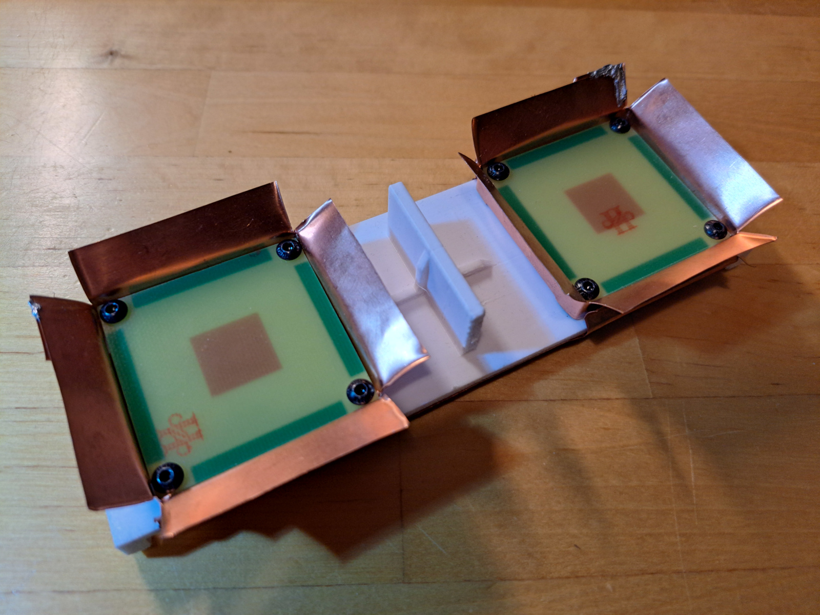
TX and RX patch fed horn antennas.
However, more gain would be good to have for improving the signal-to-noise ratio. Sidelobes at 90 degree angle should also be lower to decrease TX-RX leakage. To solve this I added a sheet metal horn structure around the antenna, making it a stacked patch fed horn antenna. The horn increases the height by 10 mm, but even just a sheet metal wrapped around the patch gap increases the gain and decreases sidelobes without increasing the height. I haven't found a similar structure in any publications, but it wouldn't surprise me if some exist, as it does seem straightforward.
A pyramidal horn with filled-in corners would likely offer slightly higher gain and be mechanically stiffer than this four-flap design. However, this was easier for me to manufacture. I cut the copper sheet by hand with scissors and soldered it to keep it together.
This antenna has everything I wanted. It's dual-polarized, has very wide bandwidth, good gain, isn't as tall as similar gain horn antenna fed with coaxial-to-waveguide transition, and it's cheap to manufacture requiring just two FR4 PCBs, some copper sheet and few bolts and spacers. FR4 is lossy and gain would likely be around 0.5 - 1.0 dB higher if a proper low loss RF material was used, but the cost would be about 100x higher in prototype quantities and it doesn't make sense for me to spend so much more for so little improvement.
Between the antennas is a small 0.25 x 0.5 wavelength wall that decreases TX-RX coupling. I tested few different size walls and this small wall is more effective than no wall and also more effective than taller walls.
Not counting the SMA connectors, the height of the antenna is 18 mm, of which 10 mm is the height of the horn above the suspended patch. Total height including the SMA connector is 28 mm. Patch substrate dimension is 45 x 45 mm and the horn aperture is 65 x 65 mm.
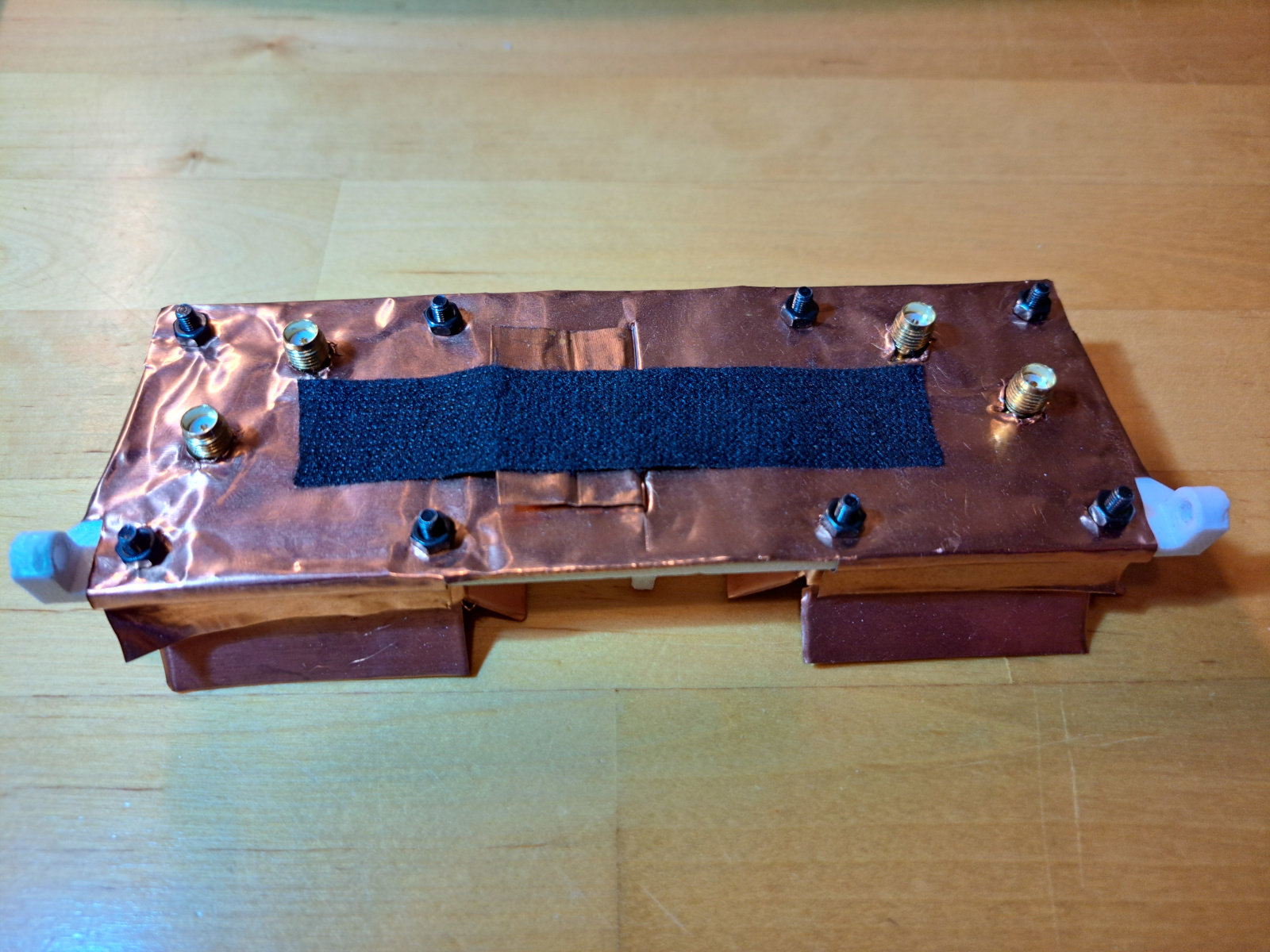
Backside of the antennas. Each antenna has two SMA connectors, one for H and other for V polarization.
Backside of the antennas is covered by copper sheet to decrease the backwards radiation. This is needed because antennas are mounted right on top of the radar PCB which doesn't have any shielding. Without shielding TX antenna backwards radiation would increase the TX-RX coupling. Copper sheet is also inserted into the wall between antennas and the tape keeps it in place.

Simulated radiation pattern of the antenna.
The simulated -3 dB beamwidth is 50/60 degrees in 0/90 degree angles. H and V feed slots are rotated 90 degrees and the radiation pattern from the other port is similar but rotated 90 degrees. Simulated peak gain is 10.0 dB.
Sidelobe to 90 degree direction is about -10 dB. It's important for this to be low to minimize TX-RX leakage.
Since the antenna radiation pattern isn't quite symmetrical, mounting the other antenna at a 90-degree rotation compared to the first one ensures good antenna pattern matching between HH and VV polarizations. If the TX antenna transmits H polarization from the first port, RX antenna receives H polarization from the other port, and other way around for V, causing the two-way antenna pattern to match between the both cases. However, HV and VH antenna patterns don't match the HH and VV patterns, since in the cross-polarization case the same port is used to transmit and receive on both antennas.

Measured S-parameters of the antenna.
There is a slight difference in the H and V port matching due to their slightly different coupling slot sizes. Antenna useable bandwidth is from about 4.5 GHz to 6.2 GHz which is more than enough for this application.
Mechanical design
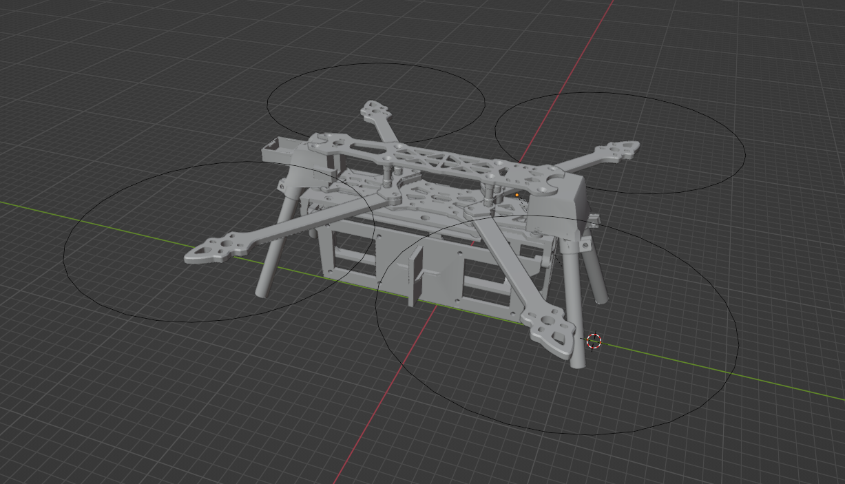
Drone mechanical model in Blender.
The drone needs some mechanical parts to hold the radar on the drone frame. The flight controller is mounted inside the frame, but there isn't enough room inside it for the radar, so I designed a 3D printed mount that holds the radar PCB under the drone frame. This mounting position also requires landing legs so that the drone doesn't land on the radar. I designed it in Blender since I don't know any mechanical CAD programs. It works just fine for these simple parts.
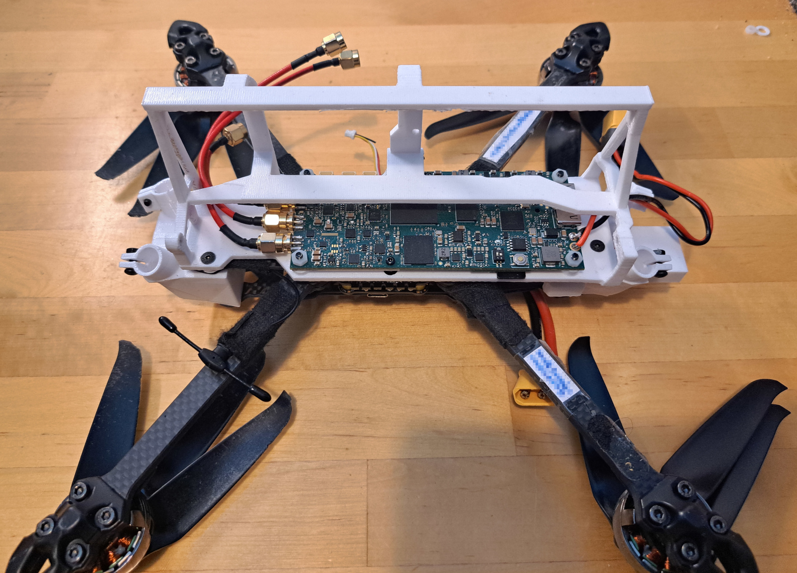
Radar attached under the drone.
The radar mount holds the radar PCB on the drone frame. It would be a good idea to have some sort of weather proof enclosure for it, but I haven't got around it yet. I added some material over the PCB to protect it in case the landing legs fail.
Radar holder attaches with four screws to the drone. Drone radio controller antenna is visible at the bottom left. Propellers are collapsible, these make it much easier to transport the drone as with these it fits in a backpack.
Receiver polarization switch PCB.
Antenna board is held with two bolts that allow its angle to be changed. Flight controller serial port is attached to one of the JST connectors. There also other JST connector from flight controller that is currently unused and just held with tape in place.
Transmitter has polarization switch and two SMA connectors on the PCB, but the receiver polarization switch is on a separate PCB due to lack of space. I had a mounting holes for it on the radar holder part, but the SMA cables are stiff enough that I found it easier to just leave it hanging there. Polarization switch connects to the radar PCB with another JST connector.
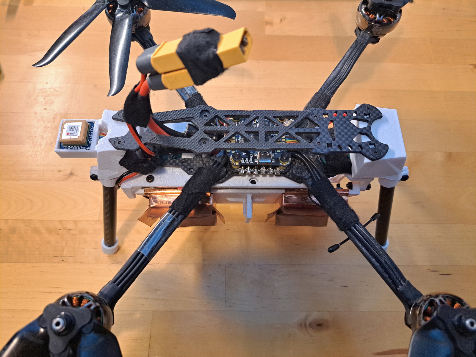
Drone with landing legs.
Landing legs are 10 cm diameter carbon tubes with 3D printed TPU caps. Smaller diameter tube would have likely been fine, these are very stiff and something else would fail before them if they are stressed too much in landing.
Radar is powered directly from the drone battery. XT60 splitter is used to connect both flight controller and radar to the same battery.
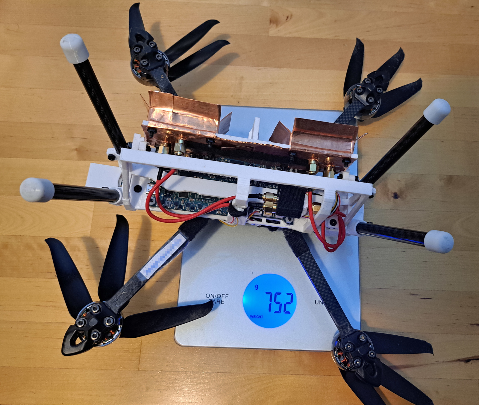
Drone balanced on a kitchen scale.
Weight of the drone without battery is just 752 grams (1.66 lbs). I have two six cell LiPo batteries, the smaller 1300 mAh capacity battery weights 196 grams and the bigger 2200 mAh battery weights 322 grams. With the smaller battery the total weight of the whole system is just 948 grams.
Image formation
Radar measures the distance and phase of each target. To convert these measurements into a radar image, matched filtering can be used. For each pixel in the image, generate a reference signal corresponding to what a target at that position would reflect. Multiply the measured signal with the complex conjugate of the reference signal for each measurement, then sum these products over all measurements. When the measured signal closely matches the reference signal, their product becomes large because the phases align. If it doesn't match, the result of the multiplication is a complex number with a random phase, and summing random complex numbers will average out generating a low response.
The image formation can be written as:
, where \(\mathcal{P}\) is the set of pixels in the image, \(N\) is the number of radar measurements, \(S_n\) is Fourier transformed measured IF signal \(s_n\), \(d(p,x_n)\) is the distance to location of pixel \(p\) from radar position at that measurement \(x_n\), and \(H^*\) is complex conjugate of the reference function of what target at that position in the image should look like (Fourier transform of the radar IF signal from target at that position in the image).
This is called backprojection algorithm. It's simple and doesn't make any approximations or assumptions about flight geometry, but it's very demanding to calculate. For example with 1 km x 1 km image with 0.3 m resolution and 10,000 radar sweeps, calculating the image needs \((1000/0.3)^2 \cdot 10000 = 111 \cdot 10^9\) backprojections. This means over 100 billion complex exponentials and square root calculations is needed for one image, and image size and number of sweeps can be even larger in practice. There are some clever algorithms that can be used to speed this up, but they often have approximations or only work with linear flight tracks. One easy improvement that can be made without many drawbacks, is to use polar coordinates instead of Cartesian coordinates, as that requires less pixels in the image since angular resolution is constant while cross-range resolution is better closer to the radar. Polar coordinate image can then be afterwards interpolated to Cartesian grid.
1 2 3 4 5 6 7 8 9 10 11 12 13 14 15 16 17 18 19 20 21 22 23 24 25 26 27 28 29 30 31 32 33 34 35 36 37 38 39 40 41 42 43 44 45 46 47 48 49 50 51 52 | |
Some years ago this would have been unbelievable amount of compute, but with modern GPU this can be calculated in under a second. This problem is especially well suited for GPU implementation since every pixel can be calculated independently in parallel. Very straightforward CUDA kernel is able to calculate 220 Billion backprojections per second on RTX 3090 Ti GPU. This is very respectable speed considering that each backprojection requires square root and complex exponential (which can be calculated with just sin and cos). I'm sure that someone experienced with CUDA programming could make this even faster as this doesn't have any optimizations or approximations and is just the direct algorithm implementation.
Autofocus

Autofocus block diagram.
Positioning accuracy of the GPS and IMU isn't good enough to form a high-quality image. Ideally, the position should be known to a fraction of the wavelength, but accuracy of the GPS isn't good enough. To achieve good image quality, an autofocus algorithm is necessary to focus the radar image using information from the radar data.
The most commonly used autofocus algorithm is phase gradient autofocus. It's simple and fast autofocus algorithm that works by taking an unfocused radar image as an input and solving for a phase vector that when multiplied with the azimuth FFT of the image gives a focused image. However, it doesn't work well in this case since the azimuth beam is wide and the radar baseline is long causing the focusing errors to be spatially dependent.
I updated my previous backpropagation autofocus to use PyTorch and made some improvements. This autofocus algorithm works by forming the radar image, calculating the gradient of the input velocity, and clipping the learning rate to limit the maximum position change to a predefined value. The input velocity is then updated using a gradient descent optimizer. I found that using a 3D position doesn't work well, as it often tends to just nudge each position in random directions. Instead, using velocity and integrating it to position seems to yield much better results. A small regularization term is also included to minimize the distance between the optimized and original positions, favoring smaller updates.
Adjusting the learning rate based on the maximum position change makes it easier to set the optimizer meta parameters. Instead of setting the learning rate directly, maximum position update is given which is used to set the learning rate.
This is very general autofocus algorithm that makes no assumptions about the radar system, scene, or the flight track. The obvious disadvantage is that it requires forming the radar image many times making the already slow image formation many times slower. Without the fast GPU image formation this would be too slow to be useful.
The autofocus algorithm is available on Github.
Measurements
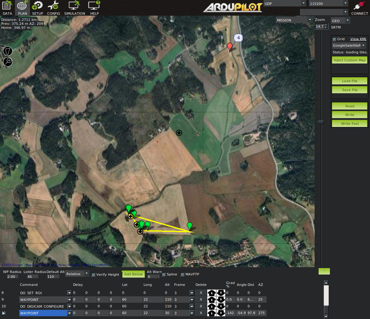
Configuring the mission in ArduPilot Mission Planner.
The mission is programmed beforehand with the ArduPilot Mission Planner. The drone will automatically fly the programmed waypoints, there are also commands to set the ROI (region of interest) so that antenna always points towards it, and the radar measurement is started with digicam configure command in the mission. It's originally meant for configuring ordinary camera, but I programmed the radar microcontroller to listen to it. Using an existing command makes it easy to make the radar work with the existing ArduPilot software.
Setting ROI, which is needed for spotlight imaging, needs a patch to ArduPilot firmware. By default drone's front will always point towards the ROI and there isn't a way to configure it to point the antenna towards ROI instead. The patch is available on the ArduPilot Github as a pull request.
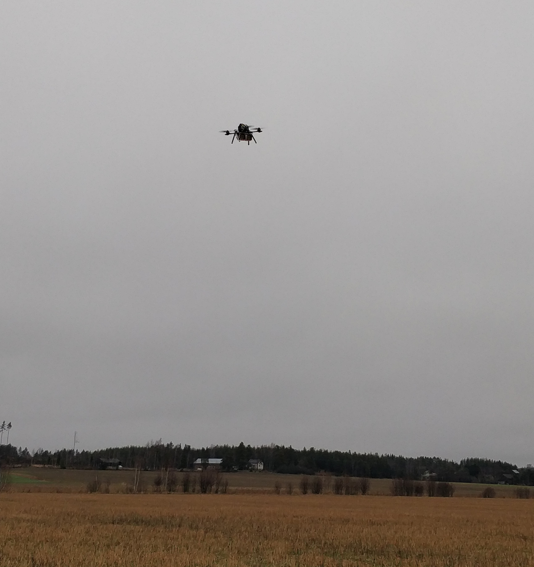
Drone in action.
The scene is a wide open field. There's about 1.5 km distance to the forest at the antenna pointing direction. The drone flies at 110 m altitude in a straight line for about 500 m at 5 m/s velocity. The radar was configured to transmit only VV polarization with 400 µs long sweep, 500 MHz bandwidth, and 1 kHz pulse repetition frequency.
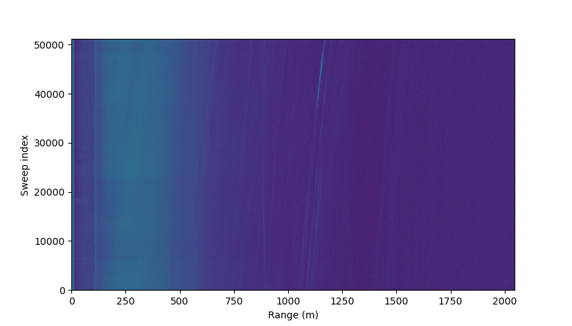
Range compressed raw data.
The range compressed (Fourier transformed) captured data doesn't look very impressive. It doesn't look anything like an image since due to the wide antenna beam at each sweep many targets at different angles are captured.
At the zero distance there is a large response from the TX-RX leakage, then the next reflection is at 100 m distance from the ground. Even though the antenna gain at directly below is much smaller than at the beam center, due to the angle of the reflection and close distance, the reflection from directly below is very large. At large distances reflections are mostly below the noise floor of individual sweeps, but during image formation many sweeps are integrated improving the signal to noise ratio. Some large individual objects are visible and their distance to the radar changes as the drone moves.
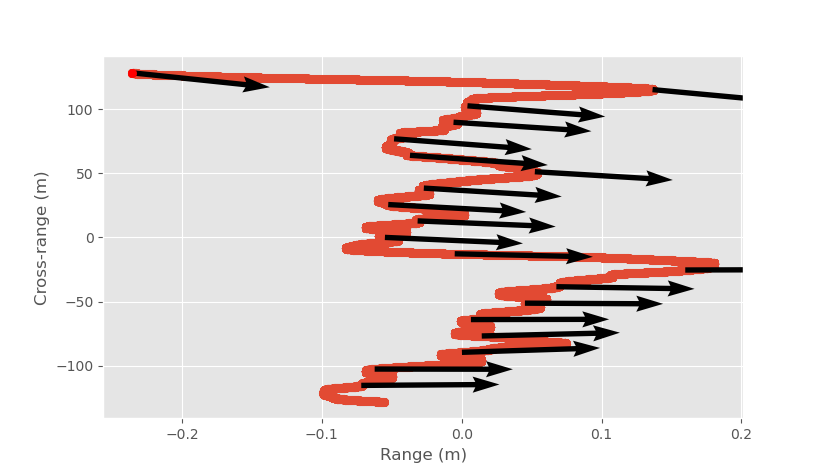
Recorded drone position and antenna pointing vector from GPS and IMU. Note the unequal axes scale.
Ideally the track should have been a straight line but there is some disturbances due to for example wind. The drone is very light and even a slight wind can easily affect it. The ROI was set quite far away there is only few degree of change in the antenna pointing direction during the measurement.
SAR image without autofocus.
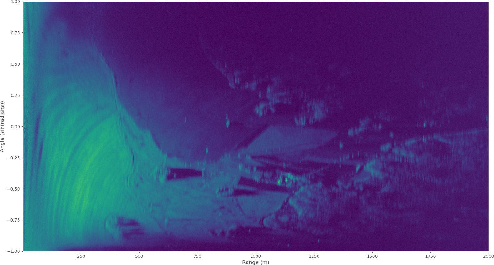
Above is the processed SAR image without autofocus in pseudo-polar coordinates that the image formation uses internally. It's pseudo-polar because angle axis is in sine of radians instead of just radians, this is slightly more efficient than ordinary polar coordinates. Image size is 6k x 20k pixels using 51,200 sweeps.
Compared to the raw data it's a night and day. Various geographical features can be now identified, but polar format makes it hard to compare to the map.

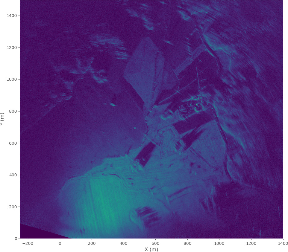
SAR image without autofocus.
Cartesian coordinate image can be obtained by projecting the pseudo-polar image to Cartesian grid. This is very fast operation compared forming the image directly on the Cartesian grid. The image is also aligned so that north points up using the drone's electronic compass measurements. Left corner is missing a small patch of data due to the rotation.
The resulting image is still quite blurry. Clearly only relying on the GPS and IMU positioning isn't good enough and autofocus is needed to get a sharply focused image.
Autofocused SAR image.
After applying 30 iterations of the minimum entropy gradient optimization autofocus, the image quality is much better. Five iterations would have been probably enough, but using more iterations does improve the quality slightly. This does take several minutes since each iteration requires calculating forward and backwards pass of the backprojection.
Due to the low grazing angle, tall structures such as trees cast long shadows. The image amplitude isn't normalized, which is why it's brighter closer to the origin. The antenna radiation pattern can be also visualized in the image. The beam center is tilted slightly to the right, and the antenna gain at the left side of the image is much smaller due to it being farther from the beam center, causing it to be dimmer.
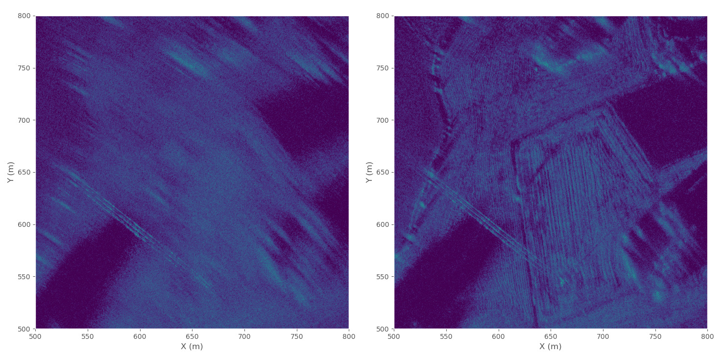
SAR image detail comparison. Without autofocus (left) and with minimum entropy optimization autofocus (right).
There is quite lot of detail in the resulting radar image when zooming in. Comparing a 300 x 300 m patch, the autofocused image reveals surface details of the field that was just blur in the image without autofocus.
I also tried using phase gradient autofocus, but it doesn't work well in this case. The result is very similar to the image without autofocus.
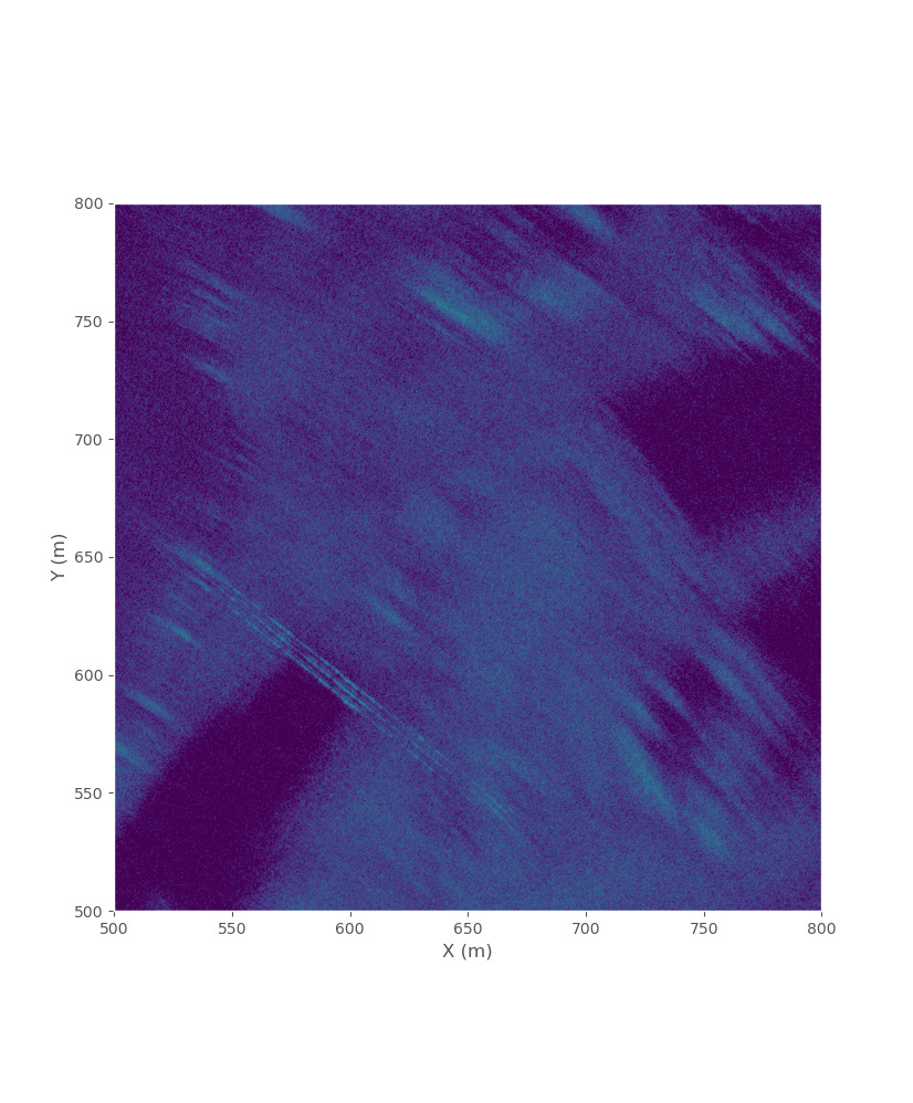
The three lines at the bottom left are power lines. They seem to be only visible in the image when the radar is looking at them at 90 degree angle, at other angles the reflectivity is so low that they are invisible.
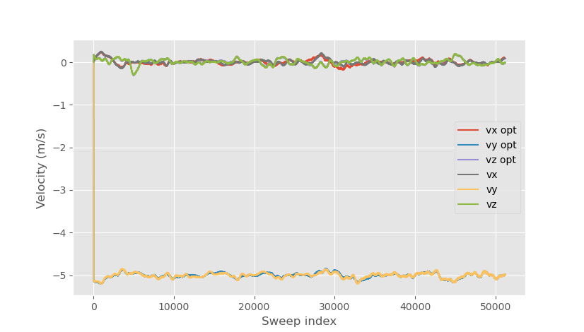
Original and optimized velocity.
Comparing the drone velocity before and after optimization the changes aren't very large. Along the track and range direction velocity components are both adjusted slightly and height direction velocity component is basically unchanged.
Full polarization measurement
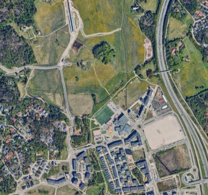
Google maps screenshot of the SAR imaging area.
I also made another measurement at other location using all four polarizations. The radar flies a linear track autonomously as before, but now the radar quickly switches between each of the four polarization switch states. Sweep length was reduced to 200 µs, pulse repetition frequency is 715 Hz for each polarization, and other parameters are kept the same. Number of sweeps in the image is the same 51,200.
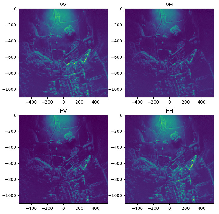
Four SAR images with different polarizations.
The four polarizations look very similar. The main differences are that cross-polarization images (HV and VH) have weaker amplitude due to cross-polarization component in general being smaller than the reflection of the same polarization.
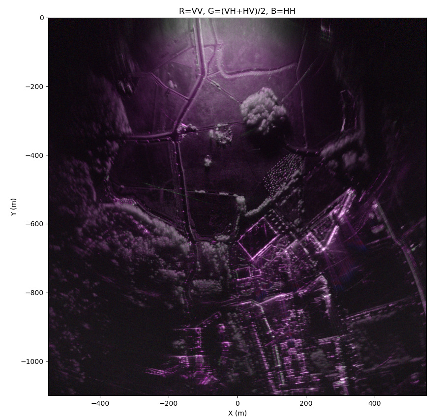
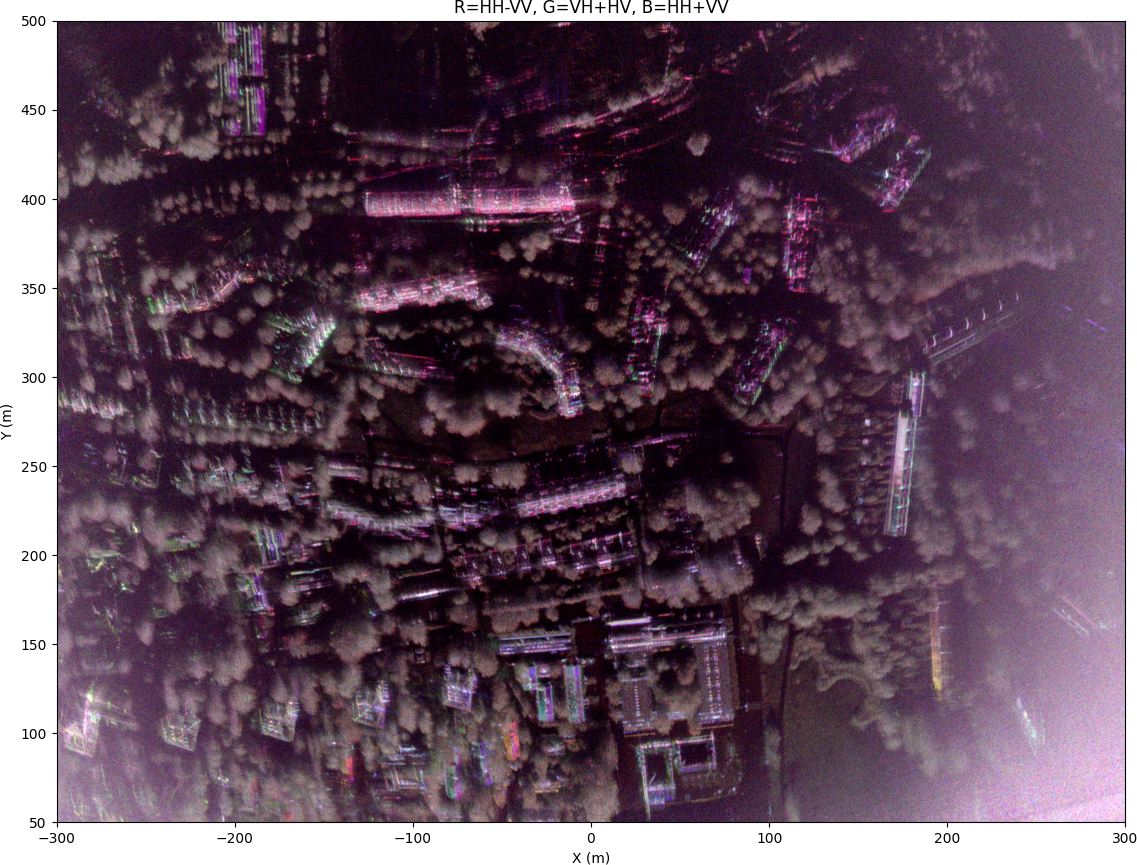
Polarized SAR image with autofocus.
Instead of looking at four different images for each polarization, it's common to use RGB color channels for different polarizations in the same image. In this colored image it's easier to visualize how each target reflects specific polarizations. The ground is tinted purple, indicating that it reflects VV and HH polarization better than the cross-polarized components. The same can be seen on the buildings and in the light poles along the road. Forest areas are colored white as they reflect all polarizations about equally. However, since the effects of the antenna radiation pattern and possibly slightly different losses for different polarization switch states are not calibrated some of the observed differences could be attributed to the hardware. Better accuracy measurements would require calibration.
The area with bunch of points around (200, 500) meters is a some kind of garden of small trees each surrounded with a metal wire mesh.
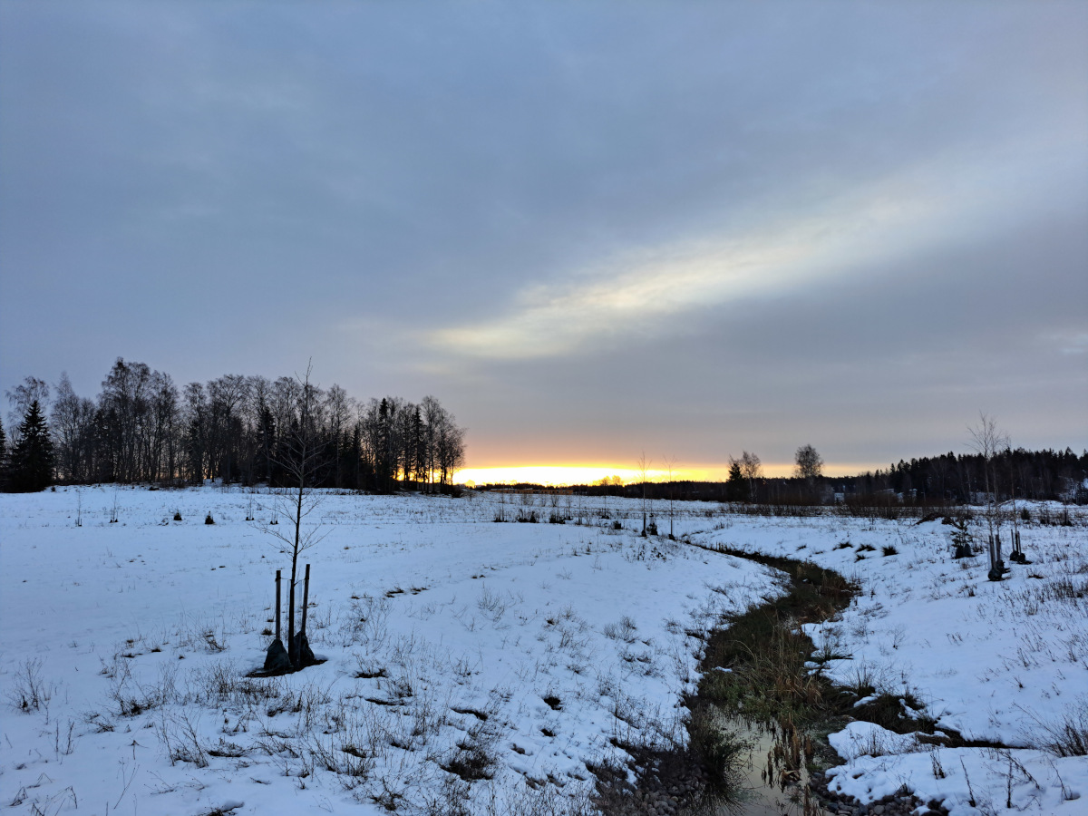
Picture at the ground at (-50, -80) m coordinates in the SAR image looking towards negative Y-axis.
There was slight amount of snow on the ground during the measurements. The visible picture is from the top of the SAR image looking down. The small forest on the left is the small patch of trees in the middle of the image.
VideoSAR
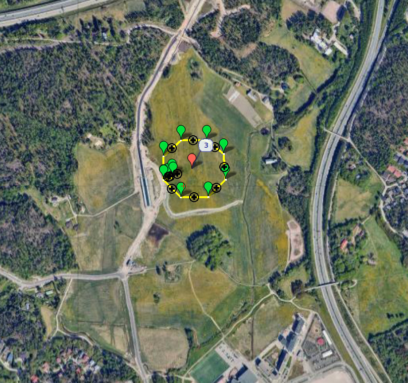
Drone waypoints for the octagonal flight path. Red marker is the region-of-interest where drone points the antenna.
The previous measurements synthesized one high-resolution image from a long baseline. It's also possible to synthesize many images with small baselines from one long measurement, and these many images can then be turned into a video.
For the backprojection algorithm, the flight track doesn't need to be linear and for this case I programmed the drone to fly octagonal track while pointing the antenna at the octagon's center.
Each frame has 1024 radar sweeps with 512 of them overlapping with the previous frame. Since each frame has less sweeps than the previous full images, the frames are noisier and have worse angular resolution. The video is sped up by about 10x. All four polarizations are used, and the image colorization is the same as in the previous polarized SAR image.
Frames are autofocused separately and there isn't any alignment of adjacent frames, which causes the frames slightly wobble or jump around occasionally. Corners of the octagon are especially challenging for the image formation since both along- and cross-range positions need to be solved accurately for a good-quality image. Angular resolution can also vary between frames as the baseline length between the frames can vary, as only the number of sweeps is the same between the frames.
Natural targets such as the ground and forest look very similar at different frames, but at several points in the video large reflections can be seen for example at bridge and power lines when they are oriented at a 90-degree angle to the radar. The bright spot that looks like it's moving at the bridge is just glint from the railing. The mismatch between antenna patterns of different polarizations is also visible as the same target can have slightly different color at the beam center or at the edge.
Imaging geometry

Radar look angle with 120 m flying height.
Without special permits, it's allowed to fly the drone at a maximum altitude of 120 m. Usually, for SAR imaging, the look angle is around 10 to 50 degrees. If the look angle is close to 90 degrees (i.e., looking straight down at the ground), the reflected power is high, but the range resolution is poor as the distance to the radar is almost the same for nearby locations. For low look angles the range resolution is good, but due to the low grazing angle the reflected power back to the radar is low. With extremely low look angle the reflected power can be about 10 to 20 dB lower than it would be compared to more usual around 45 degree look angle reducing the maximum distance the radar can see.
Another issue is shadowing caused by tall objects. For instance, when flying at 120 m height, the grazing angle at 2 km distance is only 3.4 degrees. A 10 m tall tree casts 170 m long shadow at this low angle, making it impossible to see any reflections from the ground after the tall object. This is clearly visible in all of the measurements. Especially in the full-polarization measurement only the tops of the buildings are visible at long distances.
Update October 2025
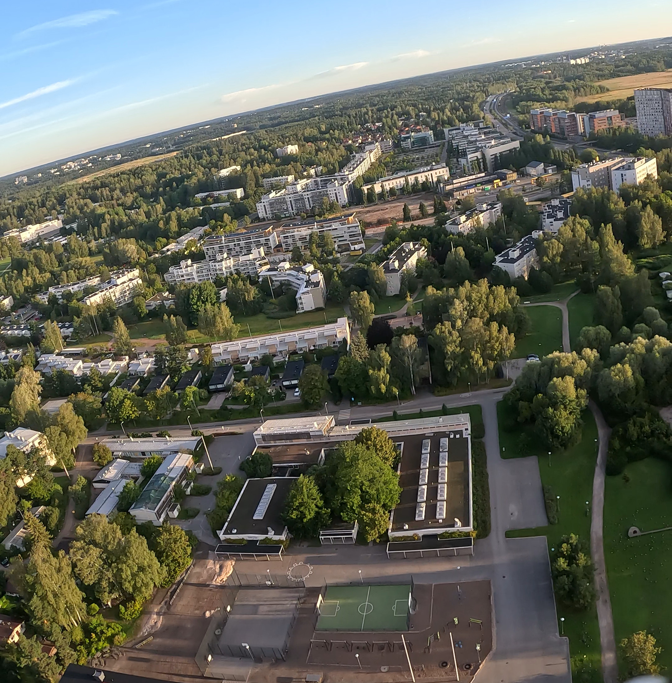
Camera image of the scene.
SAR image of urban scene with new image processing software.
Since publishing this post, I have worked a lot on the image processing software and now I can generate much better quality images. For more details see the newer post: Synthetic aperture radar autofocus and calibration.
Conclusion
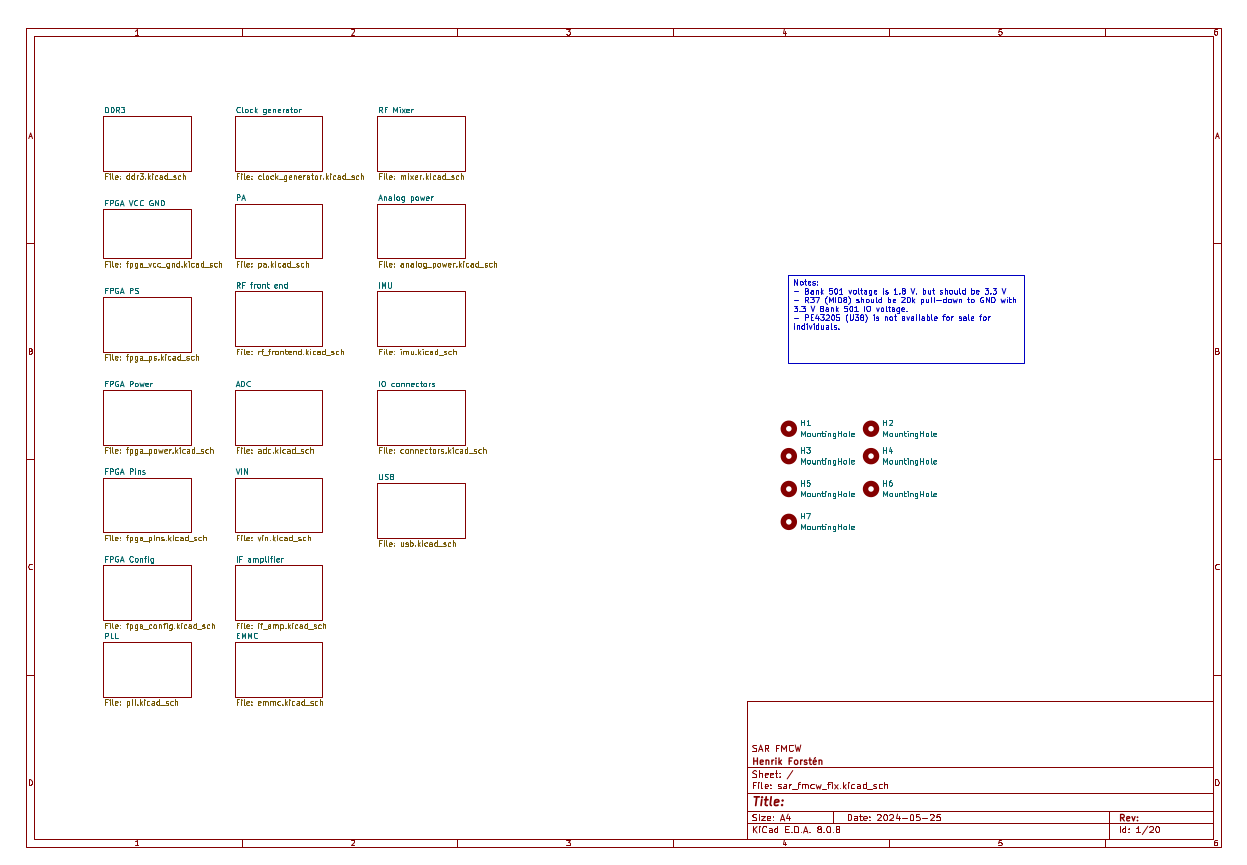
Schematic of the radar (click to open).
The synthetic aperture radar drone can image at least up to 1.5 km and likely even farther if flown higher. It weighs under 1 kg including the radar, drone, and battery. The system can capture HH, HV, VH, and VV polarizations. A gradient-based minimum entropy autofocus algorithm is capable of producing good good-quality images with a wide antenna beam using only non-RTK GPS and IMU sensor information. The total cost of the drone was about 200 EUR, 600 EUR for two radar PCBs, and about 10 months of my free-time after work. I'm very happy with the performance of the system considering its low cost.
Differentiable GPU image formation library is released on Github under MIT license. Schematic of the radar is also available above.