Introduction
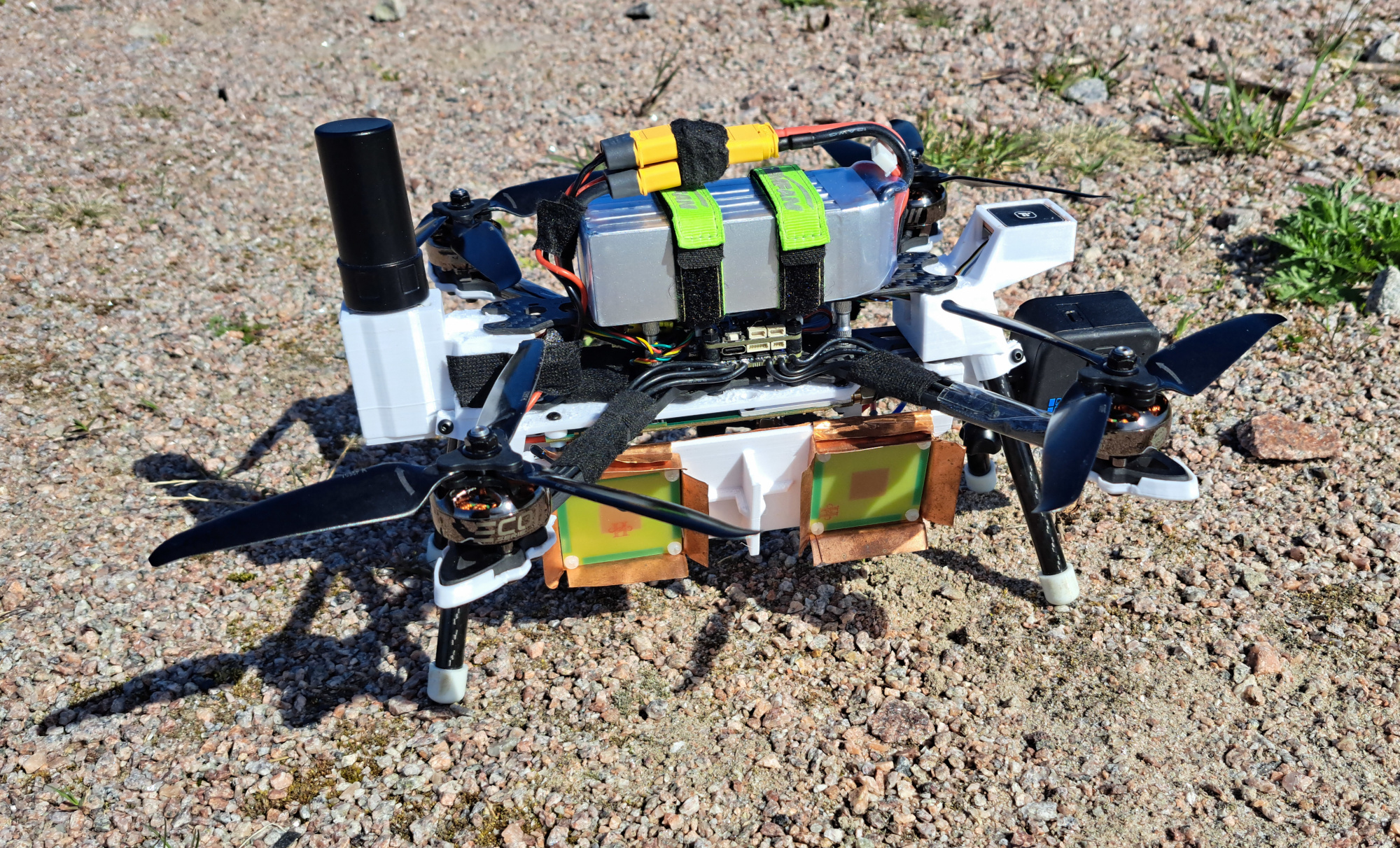
Radar drone on the ground. RTK GPS on the left side. Radar antennas under the drone, and the second GPS and GoPro camera on the right.
A year and a half ago I made my own SAR drone. Since then I have spent a lot of effort on improving both the hardware and the software. Today the image quality is much better and it's able to process interferometric SAR, all with the same very cheap radar and drone hardware.
This article goes over the changes that I made to both hardware and software to improve image quality and make interferometric SAR possible.
Hardware improvements
I'm still using mostly the same hardware I built in the initial post. Although building a new, even better radar hardware with more features and better performance is tempting, I decided to keep using the current one for now. The old hardware does have a few easy improvements to be made on both drone and radar sides.
RTK GPS
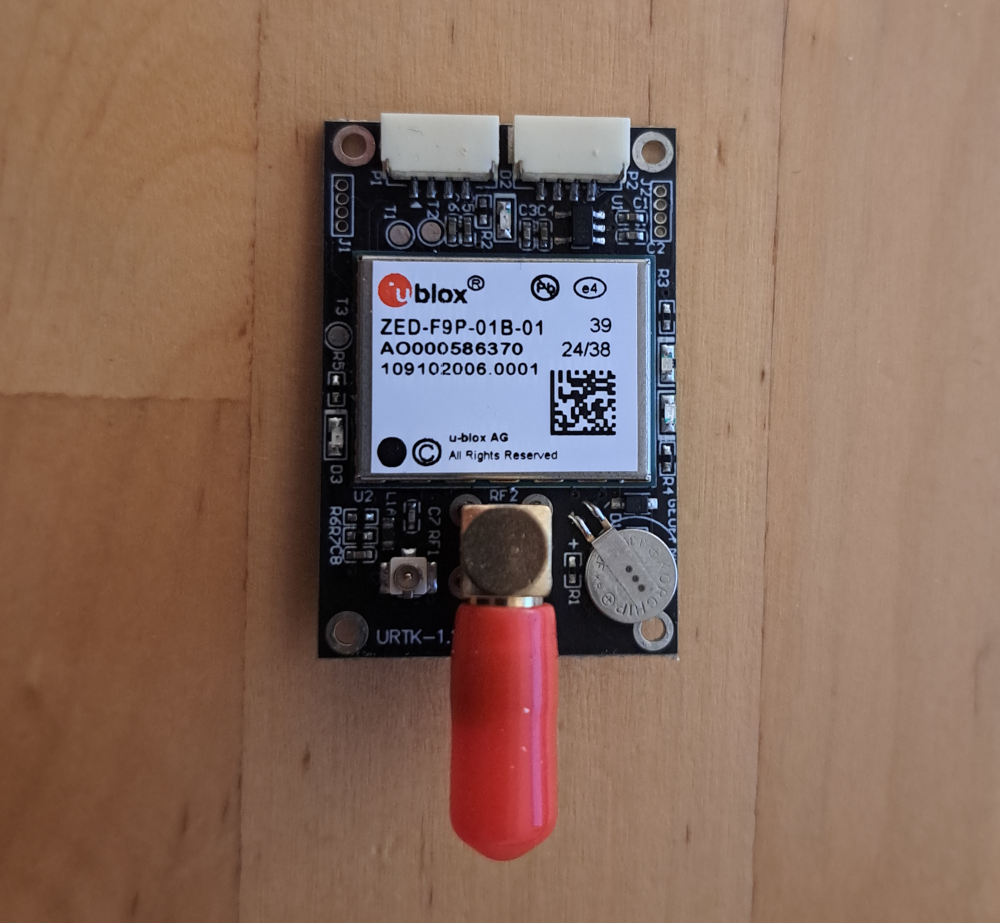
The smallest F9P RTK GPS module I was able to find.
RTK GPS uses two receivers: a fixed base station and a moving rover. The base station's location is known and stationary (if it's not known then GPS measurements over a long time period are averaged to get an accurate estimate). The base station also streams the satellite signal information (RTCM corrections) it receives to the rover. This data includes the phase of the received signal. With this information the rover GPS is able to solve for its position much more accurately, typically with 1-2 cm error, by tracking the phase of the received signals and comparing them against the nearby base station with a known location.
It was already obvious from the start that an ordinary non-RTK GPS with about 1 m accuracy is not good enough for SAR use by itself. I had to use a complicated autofocus algorithm to get a usable image with it. I complained in the initial post that there weren't any suitable RTK GPS modules that fit well into my tiny FPV drone frame. The RTK GPS modules without a PCB were quite small, for example the U-blox F9P module is just 22x17 mm, but many PCBs that have it are much larger or don't have good connections to interface with the drone flight controller. For example all the Ardusimple boards are either too large or need an external 3.3 V regulator (the flight controller has a 5V output).
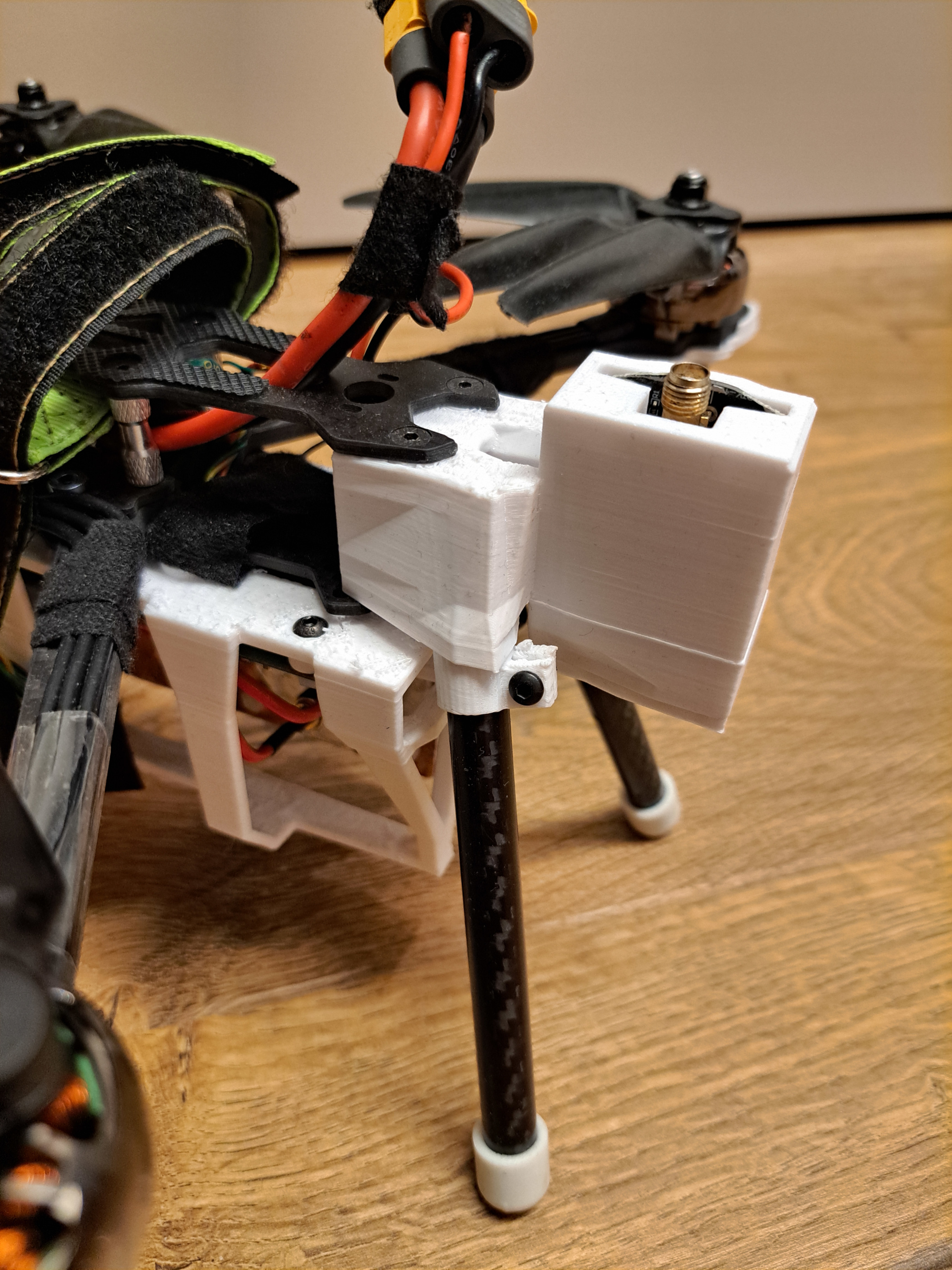
RTK GPS integrated into the drone. I designed a 3D printed piece that integrates a box for the GPS to the rear landing leg attachment piece.
Luckily I did find one suitable GPS module with an F9P chip on Aliexpress for 144 EUR, including an L1+L2+L5 frequency helical antenna (the chip only supports L1 and L2). It was a little sketchy since the listing was missing a lot of details, like the connector pinout, but I ordered it anyway. It did have an LDO for operating from the 5 V provided by the flight controller. After receiving it I traced the connector pins to the F9P pins to figure out how to connect it. I also had to file away some of the PCB because it collided with the antenna. But after all that it worked without issues.
I left the original non-RTK GPS in the drone because it had an integrated magnetometer, but the RTK-GPS doesn't have one. The second GPS also works as a backup.
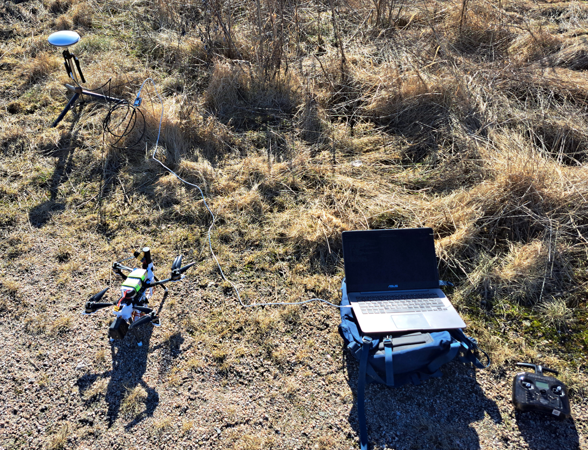
The whole system on a field: GPS base station on a mini tripod, drone, RC controller, and laptop. It all fits in the blue backpack under the laptop.
The base station is also an F9P module, but the board is different and it has a USB-C connector for easier PC connectivity. The base station antenna is also larger and better than the small helical antenna. It came with a small tripod, antenna, and the F9P module for a total of 180 EUR.
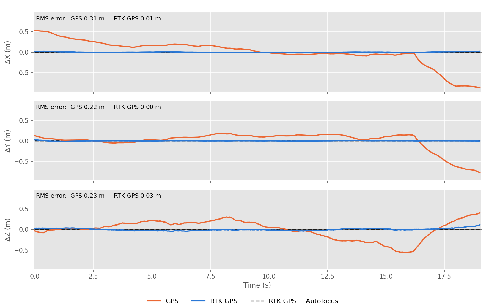
Position error vs the autofocus solution.
RTK GPS accuracy is about 2 cm compared to around 1 m accuracy for non-RTK GPS. The big increase in position accuracy helps a lot with image formation by not having to rely on autofocus so heavily. Good position accuracy is also a requirement for repeat pass interferometric SAR.
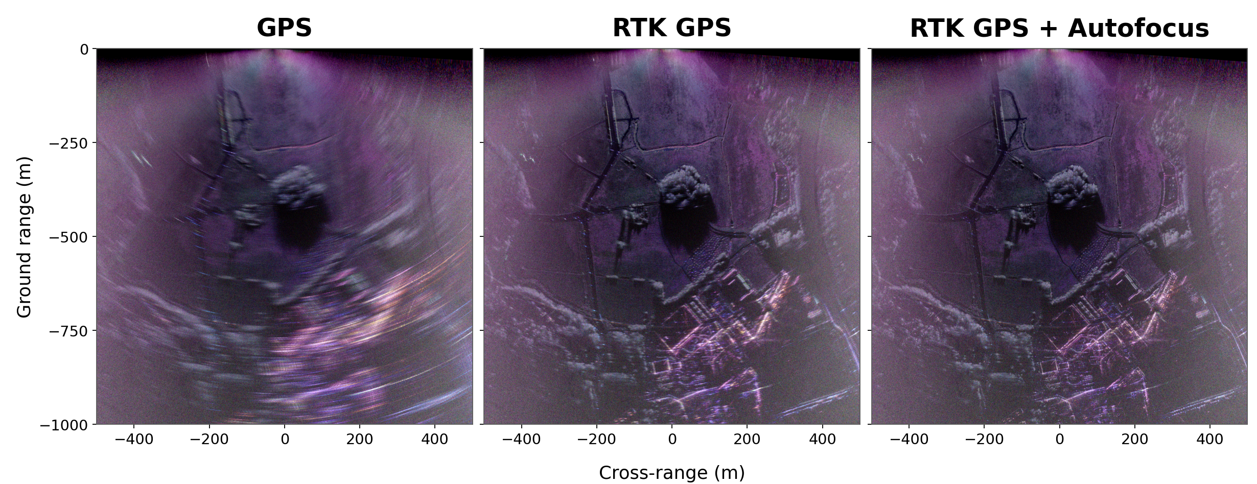
Image formation using different position references.
Comparing the images from the same measurement processed with the second non-RTK GPS, with PPK processed RTK GPS data, and with the same after autofocus shows how much the RTK GPS helps. With the non-RTK GPS and without autofocus the image is very badly blurred. Autofocus helps a little bit even with the RTK GPS. For example, the buildings at the bottom of the picture are noticeably sharper after autofocus.
PPK processing
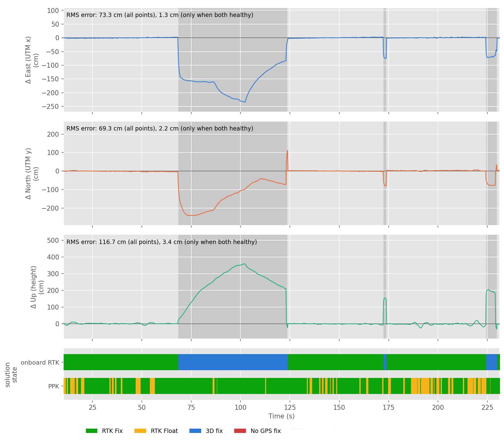
RTK position error compared to PPK processed data from one measurement where the RTK fix was lost during the measurement. With PPK processing the data remains usable since both base station and rover logs have all the required data. RTK and PPK processing seem to have different definitions for fixed vs float solutions.
While RTK is much more accurate than ordinary GPS, it's still not the best processing method possible. RTK needs real-time streaming of base station corrections to the rover and the rover processes its location in real-time. Since I process the SAR image offline, the real-time part can be dropped. This allows non-causal position solving. In Post-Processing Kinematic (PPK) positioning, both the base station's and the rover's received signals are saved. Then the processing can be run offline using the full data without caring about causality. Positions early in the recording can use information from GPS measurements later in time.
In my drone the GPS is connected to the flight controller, which has a serial connection to the radar over which position and timing information is transferred to the radar. Ardupilot documentation says that PPK processing is supported by enabling the GPS_RAW_DATA option. I did find some forum posts from people claiming to have used it successfully, but after trying it myself I found it to have multiple bugs that made it unusable. There was a fixed buffer with only room for 32 satellite measurements and any GPS measurements with more satellites were dropped. This limitation dropped practically every measurement and after fixing it I regularly saw around 80 raw measurements with good visibility. Another issue was that the signal ID (frequency band) was not logged, which made solving for the phase impossible, resulting in very poor fix quality. I fixed the issues and submitted a PR to Ardupilot so that in future versions it will hopefully work out of the box.
After the fixes I was able to use PPK processing with Ardupilot GPS raw data logging. PPK processing is especially useful if the RTK correction link had issues which would otherwise have degraded the fix quality. Initially I had a lot of problems with it. I was using ExpressLRS in Mavlink mode for the radio link and the issue turned out to be that the RTCM correction bandwidth exceeded the radio link's bandwidth, resulting in dropped packets. RC commands have priority, so it didn't affect manual control. I had to write my own RTCM server with bandwidth limitation to make sure that the radio link was not saturated. After this it worked very reliably.
PPK processing does improve the position estimate slightly even when RTK was working. The difference is about 1 cm in XY and more in Z when comparing the solutions, but the difference in image quality is minor.
PLL tuning
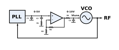
PLL with the active loop filter. Loop filter components set the bandwidth of the PLL tuning loop and affect how fast the VCO responds.
FMCW radar transmits a linear frequency sweep. On my radar this is generated by a phase locked loop (PLL). It consists of a PLL chip, a loop filter, and an external voltage controlled oscillator (VCO).
The PLL loop filter components I initially used were not tuned very well. The loop bandwidth was too wide and the PLL charge pump current was set too low. The main reason for this is that there aren't any simulators for PLLs used in a frequency sweeping configuration. Both Analog Devices and Texas Instruments have PLL simulators for their parts, but they only model fixed frequency PLLs. For FMCW radar use, the PLL constantly changes the divisor value to generate a frequency sweep and the PLL might not be locked during the sweep. Poor loop filter configuration can cause instabilities and degraded phase noise.
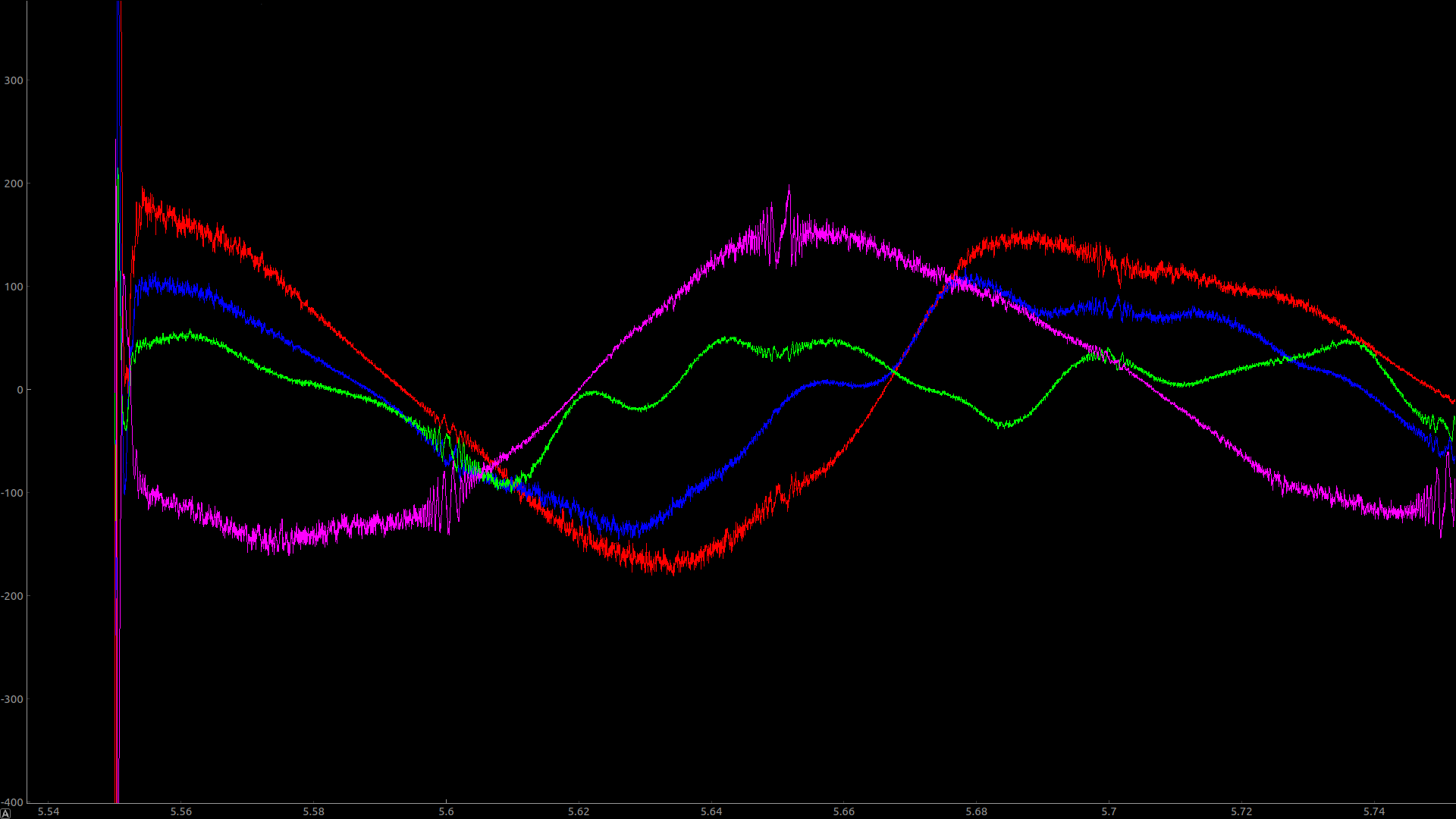
Raw ADC samples for each polarization measured indoors with a large near-range reflection and with intentionally bad PLL filter settings to maximize the IBS amplitude. Note the large spurs at every multiple of the 50 MHz reference clock. The X-axis is labeled with the instantaneous frequency in GHz. The spurs look like frequency chirps when the PLL sweeps past the fixed frequency spurs.
One type of instability is the integer boundary spur (IBS). As the PLL sweeps past an integer multiple of the reference frequency there are strong spurs at the output if the loop filter bandwidth is too wide. With an especially poor loop filter there can be strong oscillations visible in the IF signal at every reference multiple crossing. The short wideband impulses cause all range bins to have a small error which integrates in the image into straight lines with an angle depending on how their phase changes from sweep to sweep. Fixing the loop filter removed some of the straight line artifacts that were visible in the images of my previous posts. The remaining radial lines in the images are caused by RF interference.
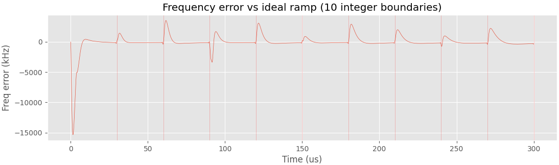
Simulated sweep non-linearity with PLL nonidealities included. The nonideality parameters are unlikely to exactly match the true hardware, but the optimal loop filter parameters should still mostly transfer over.
I made a simple PLL simulator program, with the help of an LLM, that simulates a frequency sweeping PLL with a MASH delta-sigma modulator like the LMX2491 chip I'm using has. I used it to tune the loop filter components for optimal sweep linearity. I eyeballed some numbers for the nonidealities based on the measurements I made so that the IBS amplitude looked about right, then ran the loop filter optimization. According to the simulator the optimum is a very narrow loop filter (60 kHz bandwidth and 55 degree phase margin with the sweep parameters I was testing with), with just barely enough bandwidth to be able to keep up with the sweep. Trying the solved values on real hardware gave much better performance, except that the locking time was much longer due to the low bandwidth. The longer locking time increases the time between the sweeps as the PLL needs more time to return to the starting frequency. The new loop filter also completely filtered out one of the constant frequency spurs that was visible in the IF, resulting in a much cleaner image without constant frequency spurs, lower phase noise, and much smaller integer boundary spurs.
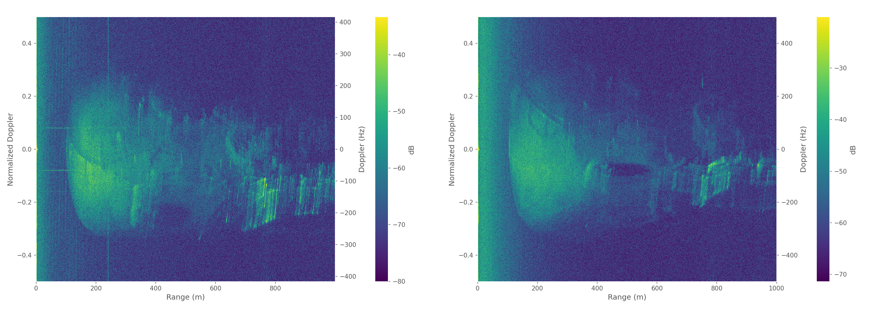
Range-Doppler maps of the raw data (2048 sweeps) without any motion compensation with the old PLL loop filter (left) and the new one (right). Note the constant Doppler and range artifacts on the left plot.
The hardware-caused artifacts are easy to spot from the range-Doppler maps formed without any motion compensation. IBS artifacts are visible as two constant-range lines at ±0.08 normalized Doppler frequency on the left image. The constant range spur is also visible at around 220 m. On the right image with the new PLL loop filter both of the artifacts have disappeared and the image is very clean. Defocusing of the scene is expected since motion compensation is not used.
Data compression
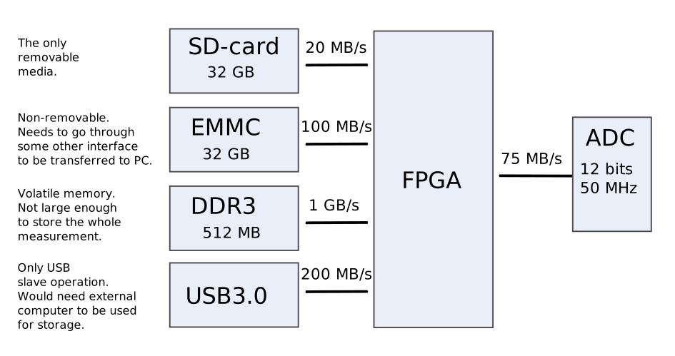
Digital interfaces of the radar. Currently the measurement data eventually needs to go to the slow SD card to be transferred out of the radar.
The data rate from the ADC is 50 million samples per second (MSPS) with each sample being 12 bits. That's 75 MB/s of data. However, the SD card interface of the Zynq FPGA only supports a 50 MHz clock with a 4-bit data bus for a total theoretical maximum bandwidth of 25 MB/s. In practice about 20 MB/s can be achieved due to overhead.
In a real measurement there is a small gap between each sweep which slightly decreases the data rate, but that is still too fast to store to the SD card in real time. I used to store the data temporarily on the EMMC during the measurement and then afterwards transfer it to the SD card to get it out of the radar. This is not ideal because a 1 minute measurement needs about 3 minutes afterwards to transfer the data from the EMMC to the SD card. That's a lot of waiting after each measurement and it would be much more convenient if the data could be stored to the SD card directly.
It could be done with hardware changes, since SD cards can support up to 100 MB/s, but the current limitation comes from the FPGA and I don't want to order a whole new PCB. I instead decided to add data compression support. I tested a few different compression algorithms and managed to get around 2.5x compression ratio losslessly. A general purpose algorithm like zstandard works well in offline tests, but the small ARM cores in the Zynq SoC don't have enough processing power for real-time compression. Even much simpler algorithms were too much for the ARM core that runs at 667 MHz. It would have a maximum of about 13 clock cycles for each sample without considering all the other tasks it needs to handle.
There are some compression algorithms specifically made for SAR data, like BAQ, but they typically assume pulse-compression data, are lossy (which could be fine if tuned correctly), and are complicated to implement. I decided to make a very simple compression algorithm just for my use case.
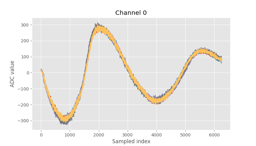
Time-domain ADC signal from a real measurement. Five consecutive sweeps overlaid.
With FMCW radar longer ranges correspond to higher frequencies, and the received power falls as \(1/r^4\) with distance. This causes the low frequency components that correspond to near ranges to have much higher amplitude than the high frequency components from longer ranges. Since low-frequency components are much stronger, the signal is mostly smooth in the time domain. Taking the difference between two adjacent samples should result in a very small value. The small values should be encodable with less bits than the raw ADC samples on average, which should allow efficient lossless compression.
This is actually quite similar to how the FLAC audio format works. First take the difference between adjacent samples, then use zigzag encoding to map the signed differences: 0, -1, +1, -2, +2, ..., to all positive values 0, +1, +2, +3, +4, .... Then use entropy coding to assign lower bit-length sequences to smaller differences that are more likely.
The choice of entropy coding is critical as it determines the compression ratio and both the compression and decompression speed. Theoretically an arbitrary variable-length code is optimal, and while arbitrary bit lengths might be acceptable on an FPGA, they are not ideal for a CPU since CPUs work with bytes and decoding would be much slower due to all the bit shifting. However, in my tests using nibble-aligned (4-bit) code widths doesn't cost too much compression ratio while being both easier to encode and much faster to decode. So the compression algorithm I ended up with is easy to implement on an FPGA, fast to decode on a CPU, and has a good compression ratio for FMCW ADC sample data.
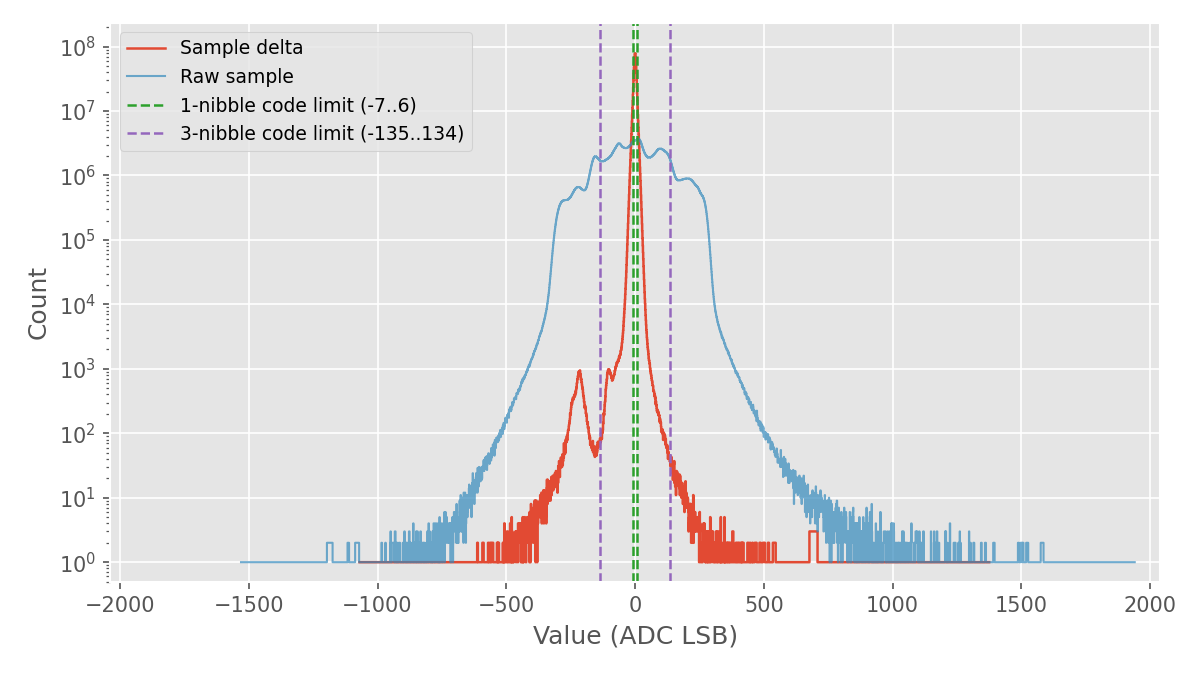
Histogram of sample and delta sizes from real measurement data. Note Y-axis log scale. 79% of samples fit in the 1-nibble code in this measurement, 20% in 3-nibble code, and only 0.004% need 5 nibbles. The small bump around -200 is from the first sample of the sweep, whose delta is calculated against 0.
After zigzag encoding, values of 13 or less, corresponding to -7 to +6 deltas, are encoded as a single 4-bit value. Zigzag values from 14 to 269, corresponding to -135 to +134 deltas, are encoded as a nibble with value 14 (E in hex) followed by one byte. 14 is subtracted from the value since codes smaller than that would have been encoded as a single nibble. This results in 12 bits used to store an 8-bit value. Larger values have a tag nibble 15 (F in hex) followed by a two byte value, requiring 20 bits to store a 16-bit value. The ADC is 12-bit so the large code does have some unused bits, but such large deltas are so rare that the slight waste doesn't matter.
| Method | Compression ratio | Bits per sample |
|---|---|---|
| FLAC | 2.8 | 4.5 |
| Rice | 2.7 | 4.8 |
| Nibble | 2.3 | 5.7 |
| zstandard | 2.1 | 6.1 |
| gzip | 2.0 | 6.5 |
Nibble is the compression method that I used. Variable bit-length encoding using a Rice code would perform better while being much more complicated to implement and slower to decode. The FLAC audio codec with max settings performs really well on this data beating all the other methods, but implementing it on FPGA in real-time is not feasible. General purpose compression algorithms perform worse here and they would also be too complicated to implement on an FPGA. The input samples have 12 bits, stored as five samples per 64-bit word for 12.8 bits per sample. The compression ratio is data dependent. If the return signal has large amplitude, the compression ratio drops. For this mission 5.7 bits are needed after compression.
FPGA stream compression
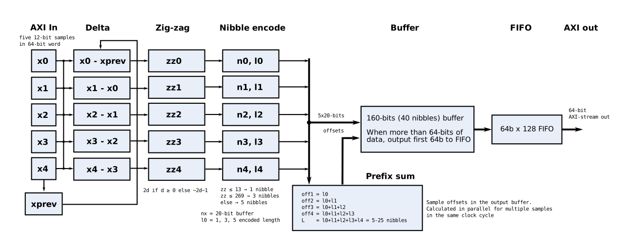
Block diagram of the FPGA stream compression.
Even though the algorithm is simple, the ARM core in the Zynq SoC is not fast enough to perform it in real time. I implemented the compressor in the programmable logic part of the FPGA instead. Only having to deal with three different codes makes the implementation much simpler. I did some premature optimization and made it process multiple samples per clock cycle. It's able to process about three samples per clock cycle. It's not quite the theoretical five samples per cycle since there are some stall cycles in the output buffer. The CPU sets up a DMA transfer from RAM to the stream compressor, which receives the samples via an AXI-stream interface, and another DMA transfers the compressed data back to RAM.
With the compression enabled the raw data rate is just about the SD card limit. I also enabled 2x decimation that halves the sample rate which makes the data rate easily fit into the SD card bandwidth limit with compression. Without decimation if the EMMC is needed for temporary storage, compression will help speed up the transfer to the SD card.
Ground control software
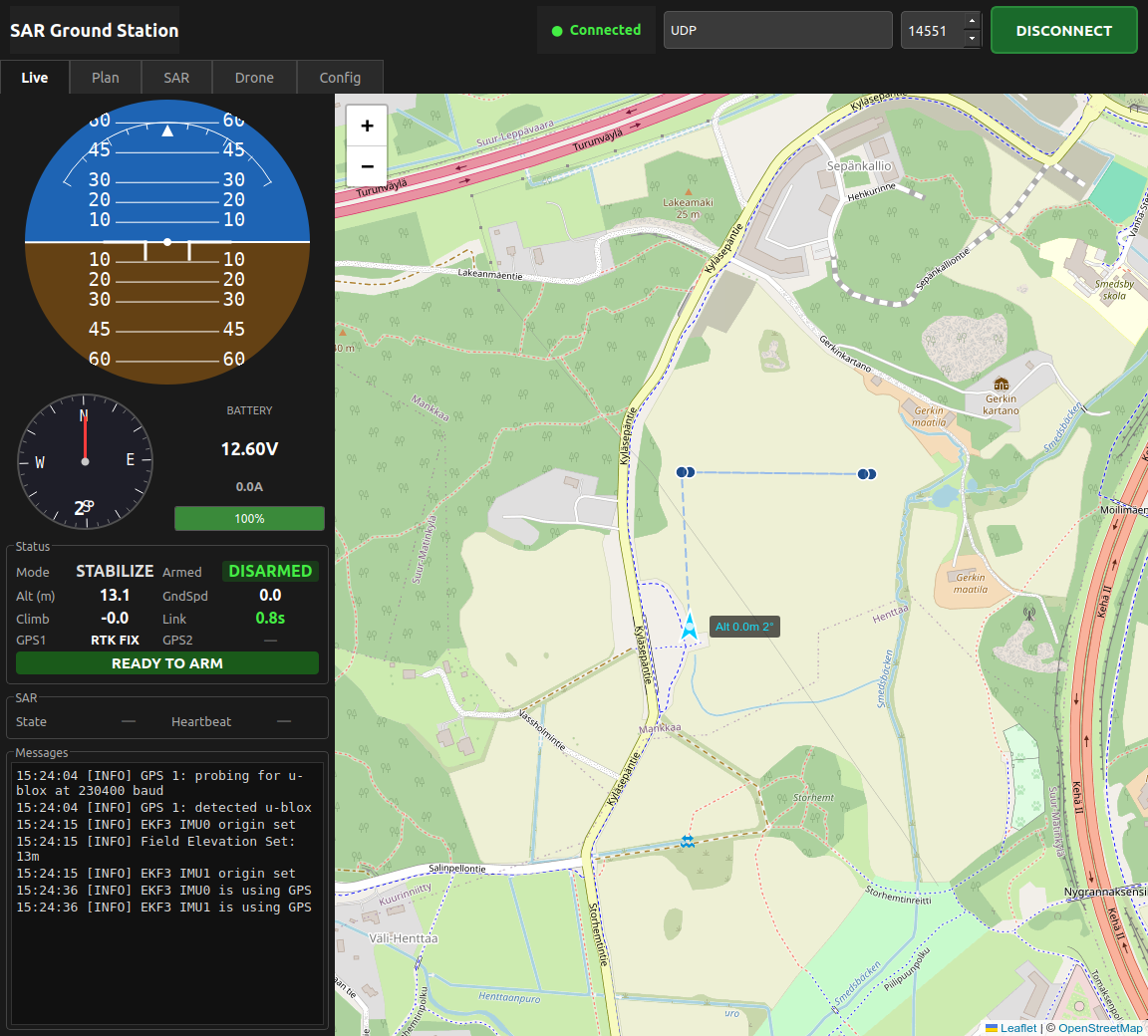
Real-time map view of the ground control software. Connected to the Ardupilot software-in-the-loop simulator in the screenshot.
I used to use Mission Planner for mission planning and real-time monitoring during missions. The main issue with it is that it's coded in C# and needs Mono to run on Linux. It's slow and crashes often. Mission planning for radar imaging is also very clumsy as every waypoint and action needs to be input manually. It is very error-prone for more complicated missions and a better alternative was needed.
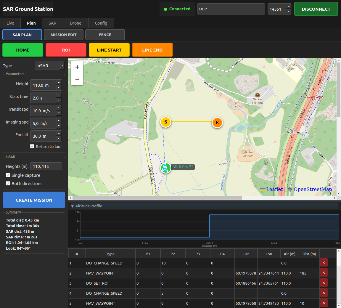
SAR mission plan generation.
I decided to make my own ground control software tailored for my radar drone. I mostly vibe coded it and I don't think I would have had the patience for it otherwise. The Ardupilot software-in-the-loop simulator was very handy in testing it to avoid having to risk crashing with the real hardware. The ground station is not safety critical as it does not control the drone during flight. All the mission critical logic is in the flight controller of the drone running Ardupilot.
It has radar mission planning that can automatically generate waypoints and actions for linear, circular and interferometric SAR missions. On another tab the radar parameters can be modified (sweep length, PRF, polarizations, etc.) and it also displays the real-time radar status. There's a tab for GPS base station RTCM correction uploading and base station log saving that also manages the telemetry link bandwidth. Another tab adjusts Ardupilot configuration parameters and there's also an option to download autopilot logs (which include the GPS raw measurements needed for PPK processing). Real-time drone location and telemetry are displayed during a mission.
Interferometric SAR
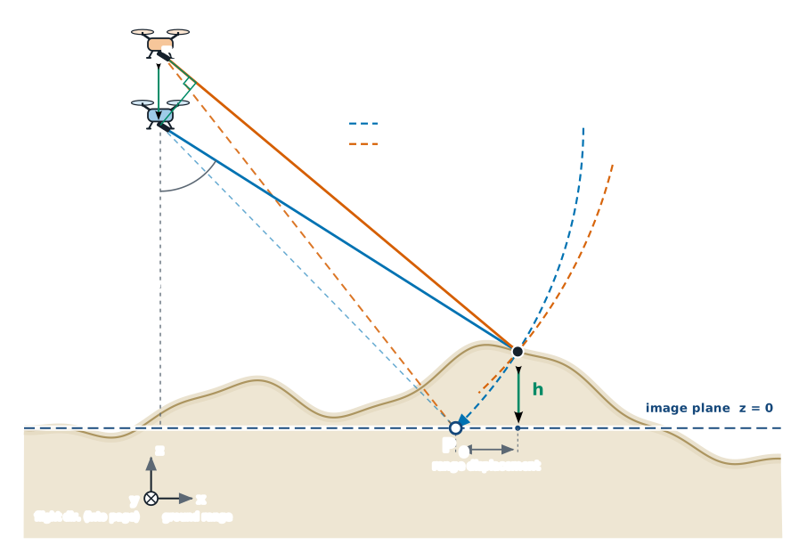
Illustration of repeat-pass interferometric SAR measurement. If the distances to the point-target can be measured accurately at two different positions, it's possible to solve for the unknown elevation of the target.
A normal synthetic aperture radar (SAR) measurement uses a single linear track at some constant height. A single linear track is not able to solve for the height of the targets, and either a known digital elevation model (DEM) is needed or it's assumed that all the targets are at zero height. If more than one measurement is made at different heights they can be used to solve for the heights of the targets with some limitations. In the above illustration the measured length difference \(B_{||}\) between the measurements depends on the surface height and it can be used to solve for the unknown surface height. However, for a real radar the distance measurement is not accurate enough, but the measured phase of the reflected signal is.
The measured phase is: \(\Delta \phi = (4\pi/\lambda)(R_1 - R_2),\ \text{mod}\ 2\pi\). It's very sensitive to distance: it changes by 360 degrees for a half-wavelength distance change and allows measuring millimeter distance differences. The disadvantage of the phase measurement is that it can only be measured modulo 360 degrees, and for a long baseline there can be multiple possible surface positions. In practice though, assuming there is only one smooth ground return allows unwrapping the phase by assuming that the phase difference between nearby positions is below 180 degrees. How well this assumption holds depends on the baseline length (a larger baseline makes the phase more sensitive to height) and the ground height variation between two image pixels.
If better elevation resolution than a single surface is needed, for example a 3D radar image of the target area with multiple resolution cells in elevation, then more than two tracks are needed to get enough vertical samples. The single linear surface approximation is good enough for many practical scenes and allows easy surface detection with just two measurements at different heights.
Backprojection interferometry processing
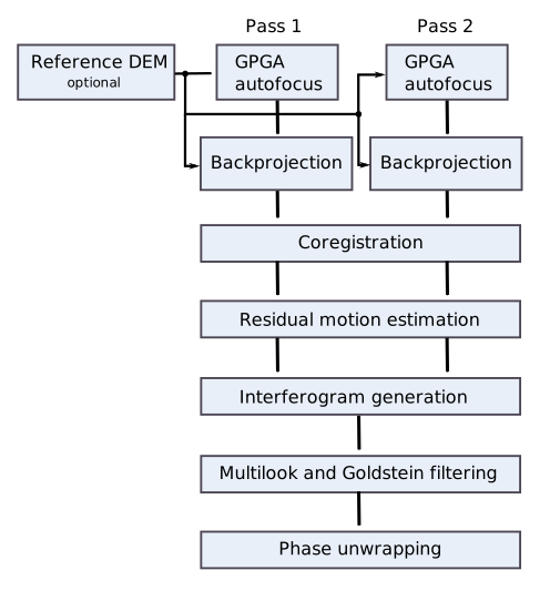
Interferometric SAR processing steps.
The interferometric SAR processing first autofocuses each image separately using generalized phase gradient autofocus (GPGA). Then each image is backprojected to either a flat ground plane or to a reference DEM. Then the images are interpolated to the same grid and residual motion estimation is run to correct for trajectory differences between the images. After that the interferogram is generated and filtered as needed. Finally, the phase is unwrapped and the elevation can be calculated from the unwrapped phase.
When a reference DEM is given the resulting output phase is the difference to the reference. This is much easier to unwrap as it is ideally zero everywhere if the measured scene matches the reference.
Classical interferometry uses images formed in slant-range geometry. However, I use backprojection that forms images on a flat ground imaging plane. This causes a slight difference in the processing steps.
Two slant-range images taken at different heights will have a flat-earth phase when imaging completely flat ground due to the slightly different ranges to the same ground patch. Backprojection on the ground plane already compensates for the path length difference, and ideal flat ground would have zero phase with any baseline.
A very good resource comparing slant-range and ground-range backprojection interferometry is "Backprojection for Synthetic Aperture Radar", by Michael Israel Duersch.
Residual motion estimation (RME)
When the two separate passes are made there will be different motion errors in them. They are autofocused separately as a first step, but the autofocus solution is not necessarily unique and it can leave a small residual phase error in the image that is not visible in the amplitude, but will have an effect on the interferogram.
There are existing RME algorithms, the best known is likely the multi-squint algorithm. Instead of using it I made a new residual motion estimation method from the same generalized phase gradient that I used for my GPGA autofocus algorithm so that I can take advantage of the raw data available in backprojection instead of working only with the images. This is to my knowledge a novel algorithm.
The backprojection image formation can be written as:
\(\mathbf{p}\) is one pixel in the image, \(N\) is the number of radar measurements, \(S_n\) is the range compressed single channel radar measurement, and \(d(\mathbf{p},\mathbf{x}_n)\) is the distance from the radar position \(\mathbf{x}_n\) at measurement \(n\) to the location of pixel \(\mathbf{p}\).
The idea with GPGA autofocus is that for a point-like target the inside term of the sum should have a constant phase when the image is focused. Averaging the solved phase corrections from many different point-like targets allows finding the common phase error and focusing the image.
For RME we want to instead make sure that the second pass phase histories for each target agree with the first pass phase histories. A naive extension of GPGA by directly comparing the two passes' phase histories doesn't work well because the sweeps are from different positions in the two images and a well-defined phase history only exists for point-like targets. For flat ground all scatterers at the same distance overlap in each measurement, which is why point-like targets are required for autofocus. However, in interferometric SAR the flat ground is what we want to align and not the point-targets.
First write the demodulated phase history of one pixel as (this is the inside term of the backprojection sum):
Then we can write the sum of the interferogram between the first pass master image \(I_m\) and the second pass slave image \(I_s\) with a per-position phase correction \(e^{-j\varphi_n}\) for the slave image data:
\(\mathcal{P}\) is the set of pixels in the image. If the interferometric phase were constant over the scene, maximizing \(J\) over \(\boldsymbol\varphi\) would immediately give \(\hat\varphi_n=\arg\alpha_n\), since every pixel contributes at the same phase.
With real topography this fails. Write \(\psi_{\mathbf p}\) for the topographic phase. Then \(\alpha_n=e^{j\varphi_n}\sum_{\mathbf p}w_{\mathbf p,n}e^{j\psi_{\mathbf p}}\), so the residual motion phase still factors out, but the remaining sum depends on the sweep index. Each sweep illuminates the scene differently, so the weights in the sum vary and pixels with different \(\psi_{\mathbf p}\) can cancel each other in the sum. The sum's phase drifts on the same time scale as the motion error being estimated, so the topography leaks into the residual motion estimate. The cancellation also decreases the estimation SNR.
However, if the sum is restricted to a block over which topography is approximately a constant, \(\psi_{\mathbf p}\approx\psi_b\), the block's phase is \(\varphi_n+\psi_b\) with \(\psi_b\) constant in \(n\). Now \(\varphi_n\) is common to every block and \(\psi_b\), which varies per-block, can be estimated and separated from it. Varying illumination only changes the amplitude and doesn't cause cancellation in the sum.
The earlier \(\alpha_n\) is replaced by a per-block \(\alpha_{b,n}\), with an additional weighting factor \(\gamma^2(\mathbf{p})\):
Two weightings are used. Per pixel, the master image is weighted by the squared power coherence \(\gamma^2(\mathbf p)\). This is used instead of normal coherence since it only compares amplitudes of the two images and is not sensitive to the topographic phase. It drops pixels with low coherence such as decorrelated vegetation and pixels outside the antenna beam. Per block, \(w_b\) measures how consistent that block's \(\alpha_{b,n}\) is across sweeps, dropping blocks with noisy phase history or where the constant-\(\psi_b\) assumption has broken down.
First, estimate the topographic phase by averaging over all the sweeps (sweeps that don't illuminate the block are dropped):
Then use that to solve for the residual motion error:
Solving the 3D position error
The same trajectory deviation method that was used in autofocus can be used here too with a few modifications. \(\varphi_n\) is the range direction error. It can be decomposed into XYZ direction errors by measuring it over many different parts of the image and then solving the 3D error.
The image is divided in the range direction into bands that are uniformly spaced in the sine of the elevation angle. Each band is tiled into azimuth blocks and solved independently. This gives \(\Delta r_{s,n} = \varphi_{s,n}\lambda/(4\pi)\), where \(s\) is the band and \(n\) is the sweep index. Then for every sweep the solutions at different bands are fitted with least squares:
where \(\epsilon_{s,n}\) is the elevation angle from the sweep position to the band center on the DEM. Bands are weighted by coherence.
Along-track error
Trying to use the same method for the along-track component works poorly and a different method is used for it instead. The along-track component of the look vector is: \(\sin\theta\cos\epsilon\), which is odd in azimuth angle \(\theta\), while cross-track and elevation components are even in azimuth.
For every band \(s\) and sweep \(n\), the block alphas are summed separately for the blocks ahead of the radar (\(\mathcal{B}^{+}_n\)) and behind it (\(\mathcal{B}^{-}_n\)):
Each sum has the common cross-track phase \(\varphi^{xz}_n\) plus the along-track phase of its side. Writing \(\bar l^{\pm}_{s,n}\) for the mean along-track look component \(\hat l_y = (y_b - y_n)/d\) over the blocks on that side, weighted by \(|\alpha_{b,n}|\),
The cross-track phase is the same on both sides and cancels in the difference, leaving only the along-track error times the lever \(\bar l^{+}_{s,n} - \bar l^{-}_{s,n}\), which is known from the geometry:
This requires an antenna beam that covers targets both ahead of and behind the radar position. For a narrow squinted antenna beam this method would fail. The split also makes the estimation sensitive to terrain and the best results are obtained if a DEM is used that removes the known terrain. In practice leaving the along-track error unsolved has the least effect on coherence and good results are obtained with just cross-track and elevation axes.
Note that unlike autofocus there is no need to pick point targets and the solution doesn't require iteration. In fact the estimate works better on flat ground than with point-like targets.
Measurements
The drone is set to automatically fly the whole measurement. The mission is programmed with the custom ground control software which also allows real-time tracking of the radar and drone status. The transit and SAR capture speeds can be set to different values. The drone could fly faster than 10 m/s during transit, but for safety I limit it to this speed. A speed of 5 m/s during capture improves the SAR image quality compared to higher speeds as more measurements can be made over the same distance. The VideoSAR in the video is post-processed, the on-board computing capability is just barely enough to get all the raw samples saved.
The two passes are flown in the same direction to make the interferometric SAR processing easier. Both passes were set to capture the same track with a 1 m difference in elevation between them. If they were flown in different directions, the velocity would cause a different Doppler phase at different azimuth bins. Also when flying in the same direction any common timing errors between the passes are subtracted away. If the two passes are flown in different directions then timing errors would not cancel. For example, each sweep is a little late compared to the GPS position tag, since the GPS is routed through the flight controller. The delay is estimated as a part of the image formation, but there is a leftover residual timing error. Between passes flown in opposite directions this would cause a positioning error, but with the same direction it cancels.
SAR image processing
The full SAR image was processed by first using GPGA trajectory deviation estimation, then fast factorized backprojection with antenna pattern weighting and a DEM. On an RTX 3090 Ti, autofocus took 22 seconds and image formation 0.9 seconds per polarization. The input data has 17,000 radar sweeps and the output image grid is 4156 x 16473 pixels. A Lee speckle filter was applied to the final output.
The reference measurement from the same area is the lidar measurement by the National Land Survey of Finland.
Full scene (1000 m x 1000 m)
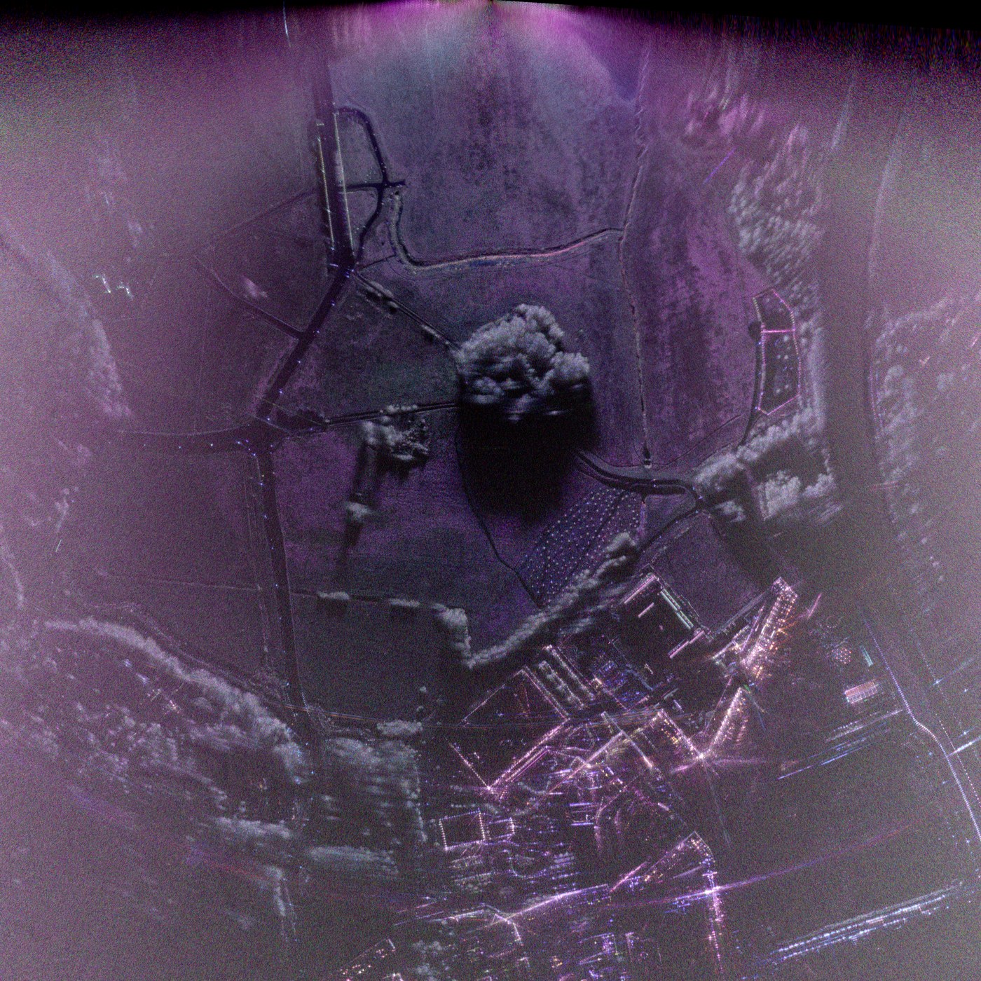 SARSatellite
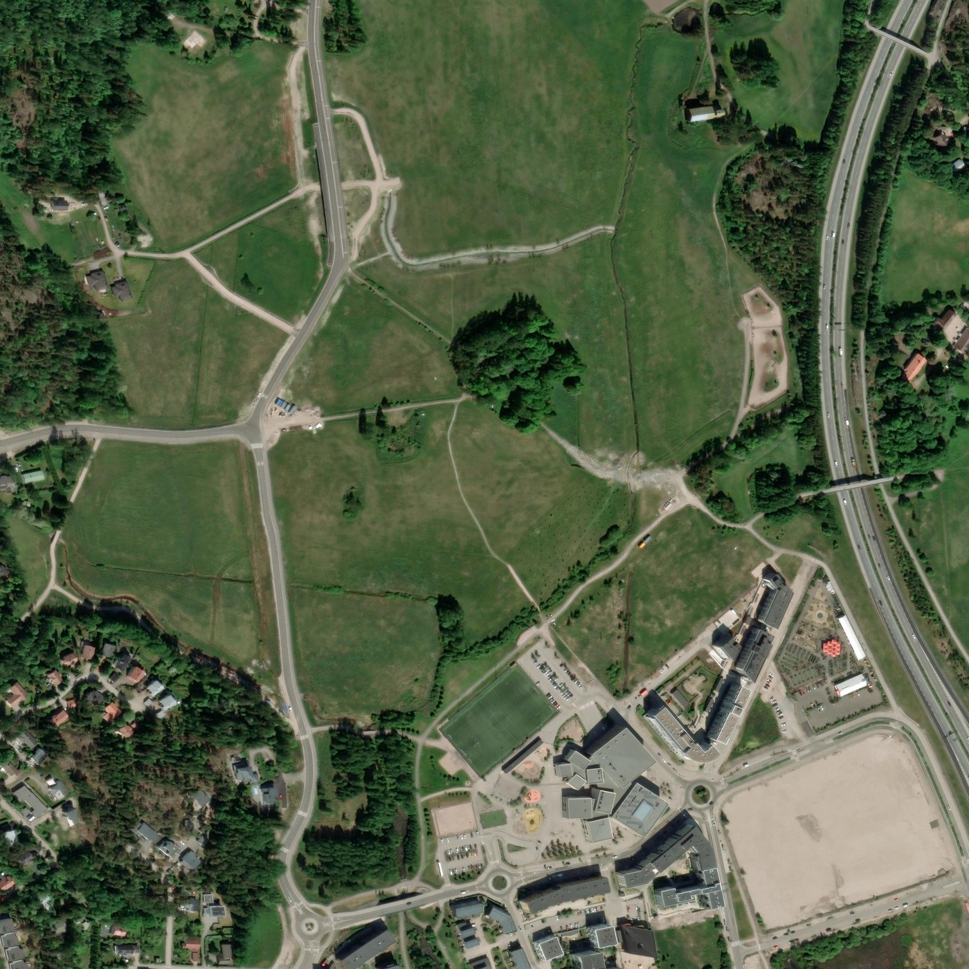
Left: drone SAR, R=HH-VV, G=VH+HV, B=HH+VV. Right: satellite imagery © Esri World Imagery.
The above image has a split view of the SAR image and a satellite image over the same area. Drag the divider to change the displayed image.
Detail (400 m x 500 m)
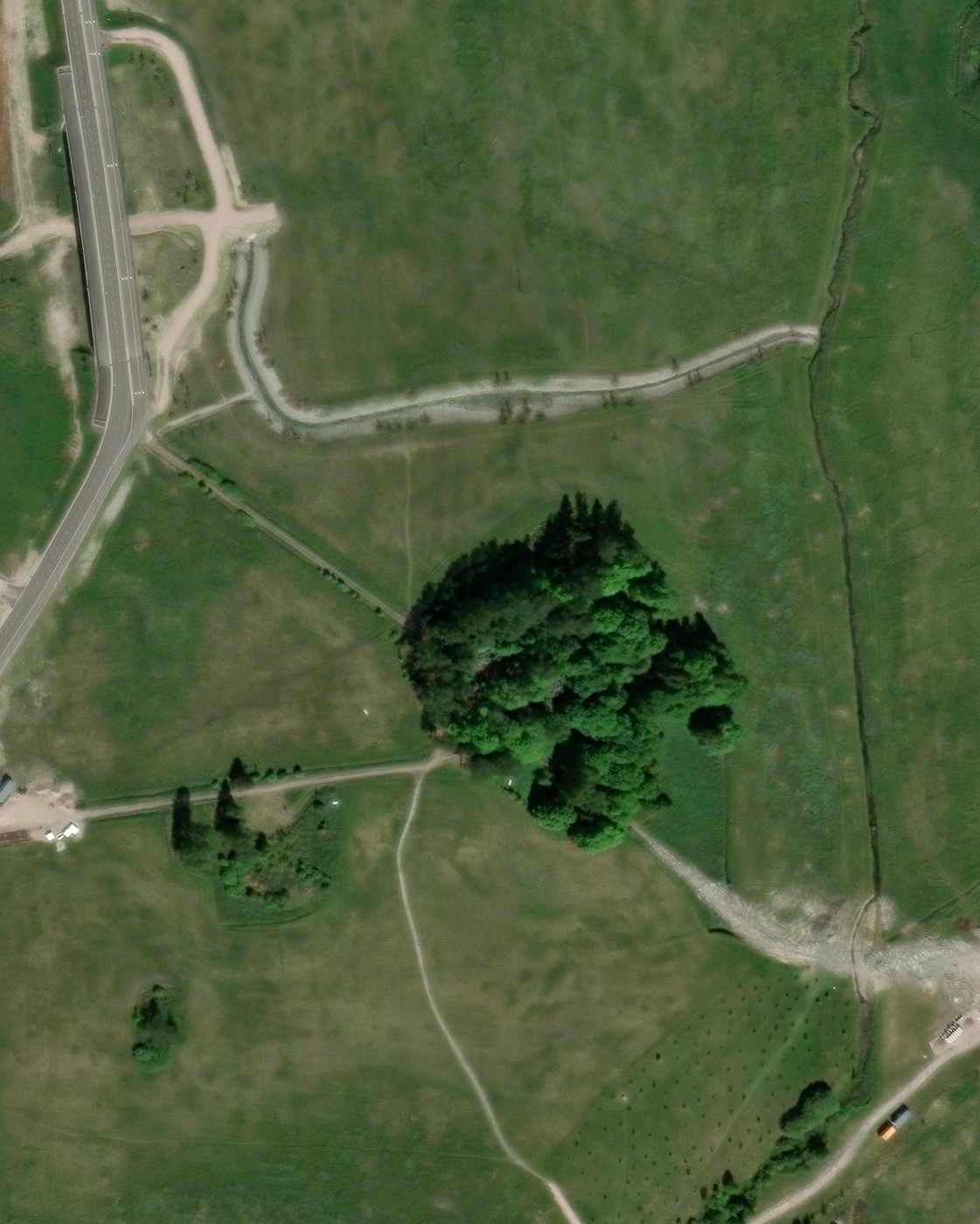
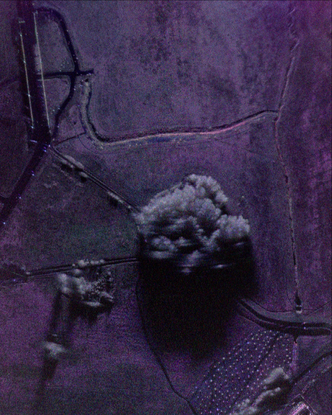 SARSatellite
Satellite imagery © Esri World Imagery.
The radar image has more detail than can be easily seen in the full scene image above. Zooming in on the field at near range shows, for example, that paths on the field are visible in the SAR image. Different surfaces can have slightly different polarimetric reflectivity causing them to have different color in the image. Light poles near the road are small enough to be barely visible in the satellite image, but are very bright in the SAR image.
InSAR processing results
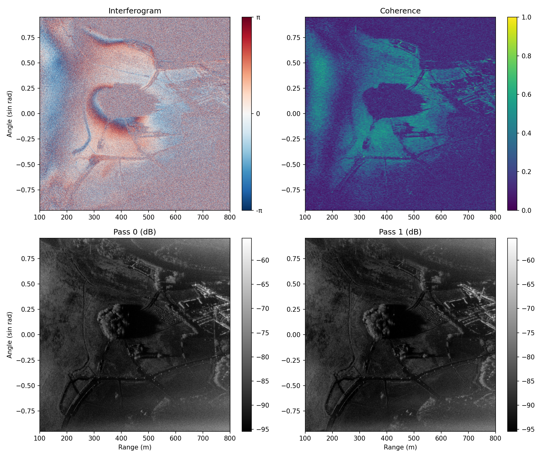
InSAR results without autofocus or RME.
When the input data is processed without autofocus or residual motion estimation the coherence is very poor, just 0.210 on average over the image. The interferogram is mostly noise at the edges although there is some area in the middle with recognizable features. Only the VV channel is used for the interferogram generation and the known baseline offset that was solved by fitting to the known DEM was removed from this image and the next ones. Without removing it there would be a both a slight azimuth and range direction ramp in the interferogram due to the coregistration error.
Although the two passes look very similar when looking at the amplitudes, there is still enough position error to cause large issues for interferometric SAR processing.
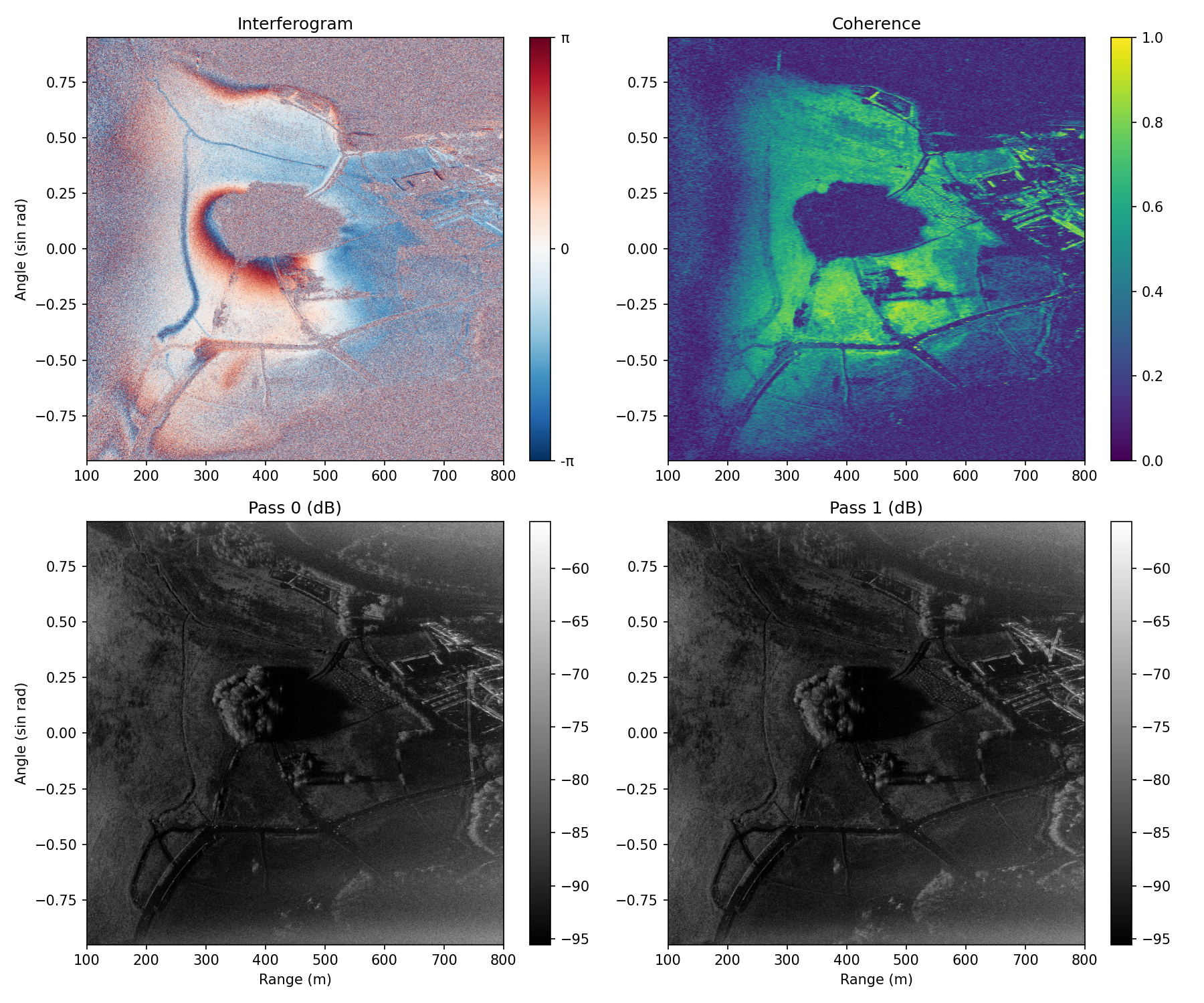
InSAR results with autofocus and without RME.
With autofocus applied to each pass individually the interferogram looks much better. Mean coherence is now 0.297 over the image. Coherence is much better than without autofocus, but especially at close ranges the coherence is still very poor.
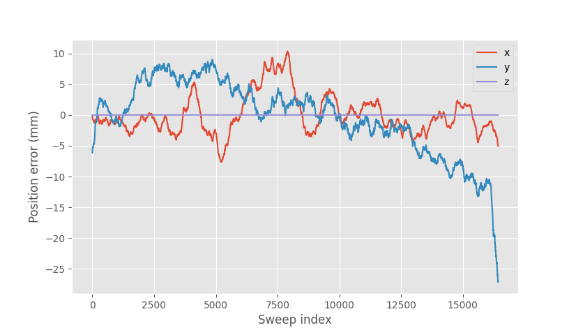
Solved autofocus correction for the first pass.
Z-error estimation was disabled and only the X and Y (cross- and along-track) errors were solved. Both passes look qualitatively similar. The range direction error is within ±1 cm, which is within the RTK GPS accuracy, and the along-track error is slightly larger at the end where the drone is decelerating.
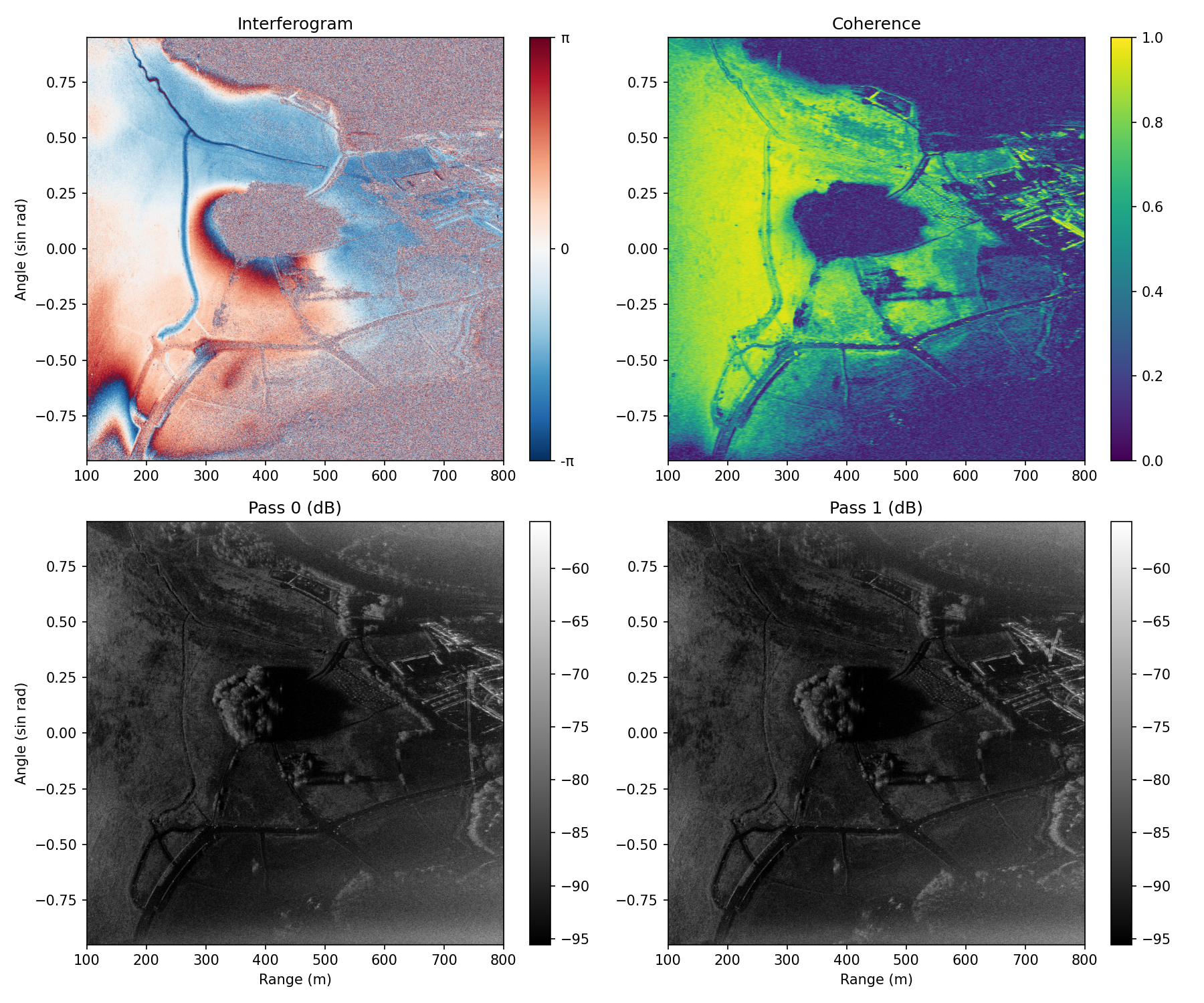
InSAR results with autofocus and RME.
With RME the results are much better. The mean coherence is now 0.453 and that includes the image edges with poor illumination and the forest regions that are decorrelated. The ground regions at near range have coherence over 0.9. The amplitude image of the second pass that was modified by RME is barely changed.
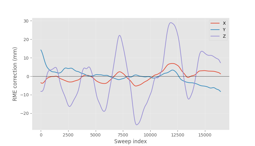
Solved residual motion error (RME).
The solved RME is mostly in the elevation direction, which is where the RTK GPS has the poorest accuracy and the direction in which autofocus was not applied.
The small forest at the center of the image and the forests at the edges are decorrelated in the interferogram. The return from the vegetation doesn't correlate between the two passes due to the large height variation. The image edges have poor coherence because the antenna beam does not illuminate them well.
All of the images so far were generated without a reference DEM, on a flat image plane placed at the take-off height based on the GPS measurement. When a reference DEM is used for image formation the interferogram directly measures the height difference of the measurement compared to the reference.
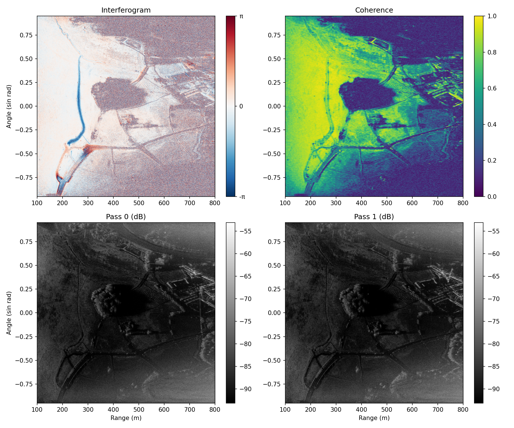
InSAR results with autofocus, RME, and reference DEM.
Coherence is 0.468, the best so far, including the decorrelated regions. The interferogram looks very different since it now measures error from the reference DEM instead of a flat plane. Areas where the measurement matches with the reference result in zero phase.
For a better comparison, open the images in separate tabs and switch between them: no autofocus, autofocus, autofocus + RME, reference DEM. In the autofocus vs autofocus + RME images there is practically no difference in the amplitude images, but the difference in the interferogram is very large especially at the near ranges. This highlights just how much more sensitive the interferometric measurement is. The amplitude images with the reference DEM are slightly different from the other images, because using a DEM for image formation corrects for layover. Without a DEM, elevated targets are imaged at an incorrect ground range.
Even in the best image after autofocus and RME, there are still low coherence areas in the image. The forest regions don't correlate between the passes, shadowed areas are not visible to the radar, and the smooth road surfaces have very little return at this look angle.
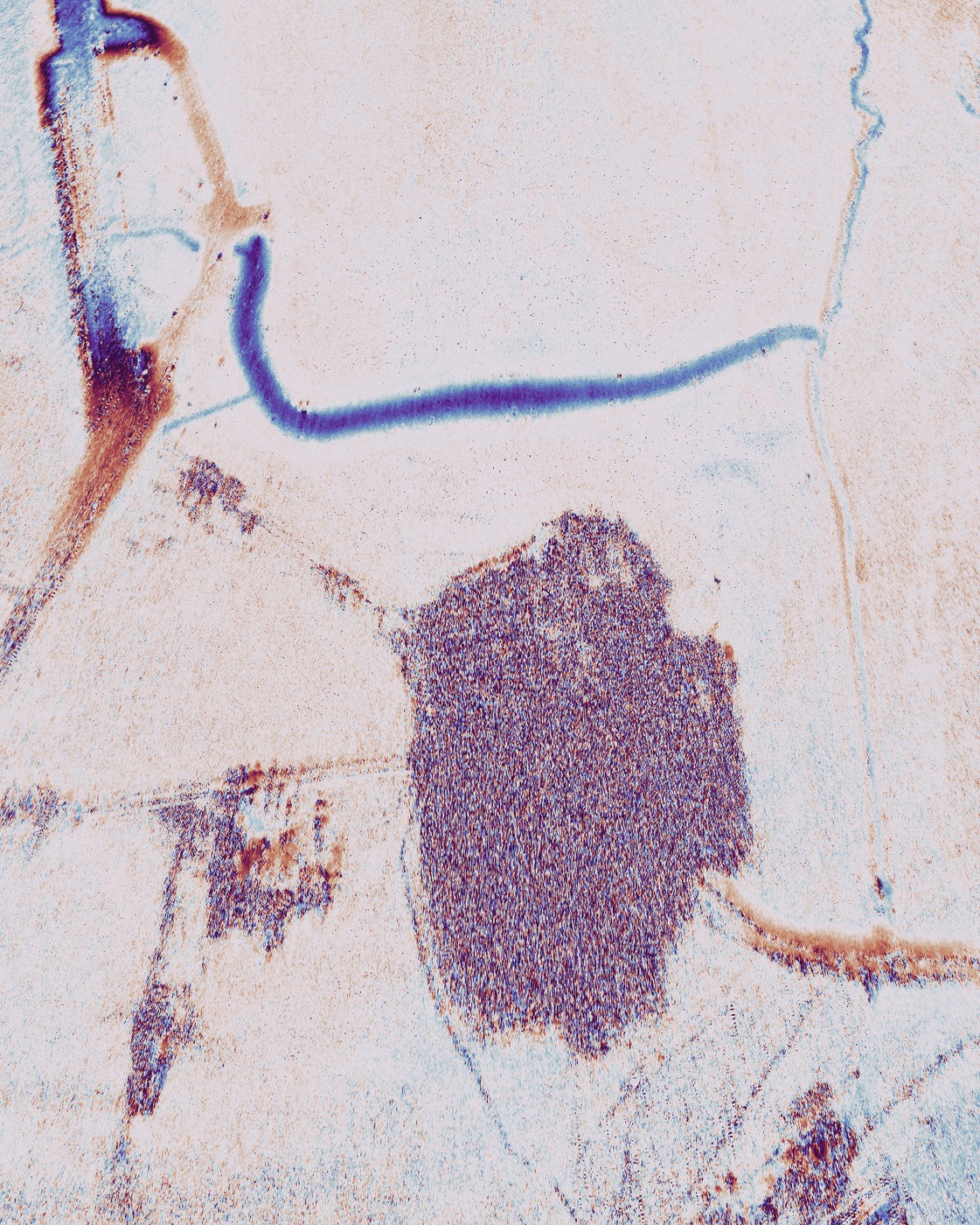 InterferogramSAR

The slider image above shows the wrapped interferogram phase on the left and the SAR image on the right. The area is cropped to the 400 x 500 m area at the center of the image that has good illumination. The interferogram is filtered with Adaptive Goldstein filter to reduce noise. It filters more where the coherence is low and less where it's high.
The interferogram shows the areas that have different height than the reference DEM. The radar and reference lidar measurements agree very well over the area. The largest differences are in the ditch at around 250 m range, the bridge near the left side, and the slightly raised road around the bottom right area. Those features aren't in the few years old lidar measurement. The bridge causes some difficulties, as the bridge and the ground under it have the same range to the radar causing them to overlap in the image. This breaks the interferometric SAR assumption that the ground is only at one height. Shadowed regions and decorrelated forest regions show just noise.
There are also structural differences between radar and lidar measurements. Lidar reflects from the top of the vegetation, but the radar signal mostly reflects from the ground surface, so the elevation measurements can be slightly different over the same area.
DEM generation
To generate a DEM from the measurement the interferogram must be unwrapped. I used SNAPHU for the 2D unwrapping. It outputs both the unwrapped phase and an estimate of the valid connected regions. The DEM is clipped to the valid region estimated by SNAPHU.
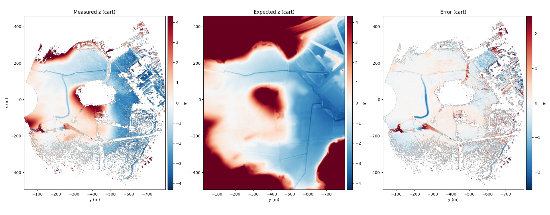
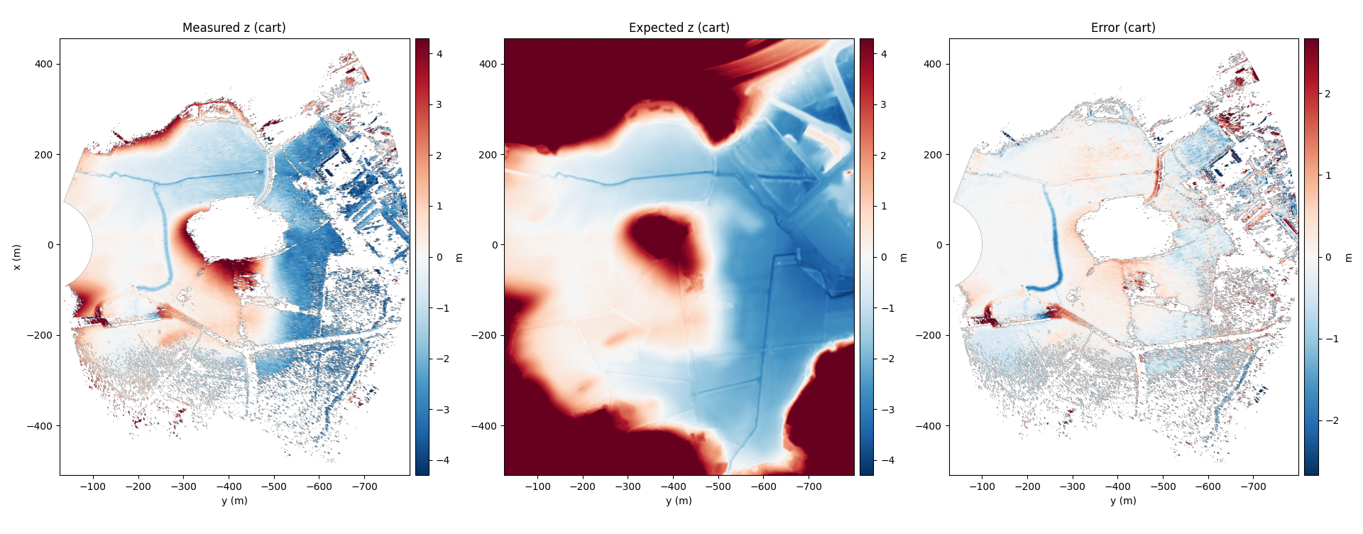
Interferometric SAR elevation map compared to the lidar elevation measurement.
There is a (9.2, 24.4, 2.3) mm error (across-track, along-track, elevation) in the measured baseline when fitted to the reference DEM which was subtracted from this and the previous measurements. The constant offset can't be solved by RME and its too small for coregistration. Without correction the baseline error would cause an elevation error of several meters at the image edges with this 1 m elevation baseline between the passes. If a reference DEM is not available, it would be possible to solve for an offset that gives a flat DEM and that would also give good results in this case.
Plotting the full radar image extent shows that the SNAPHU connected region estimation is very useful. The clipped out areas can have large errors, although there are some pixels with valid looking heights too. If the reference DEM is not used during image formation (but the constant baseline error is still solved to match the reference) the error is slightly larger near elevated regions due to layover. The ground pixels are at slightly wrong positions due to their elevation, which causes them to be compared against the wrong position in the reference.
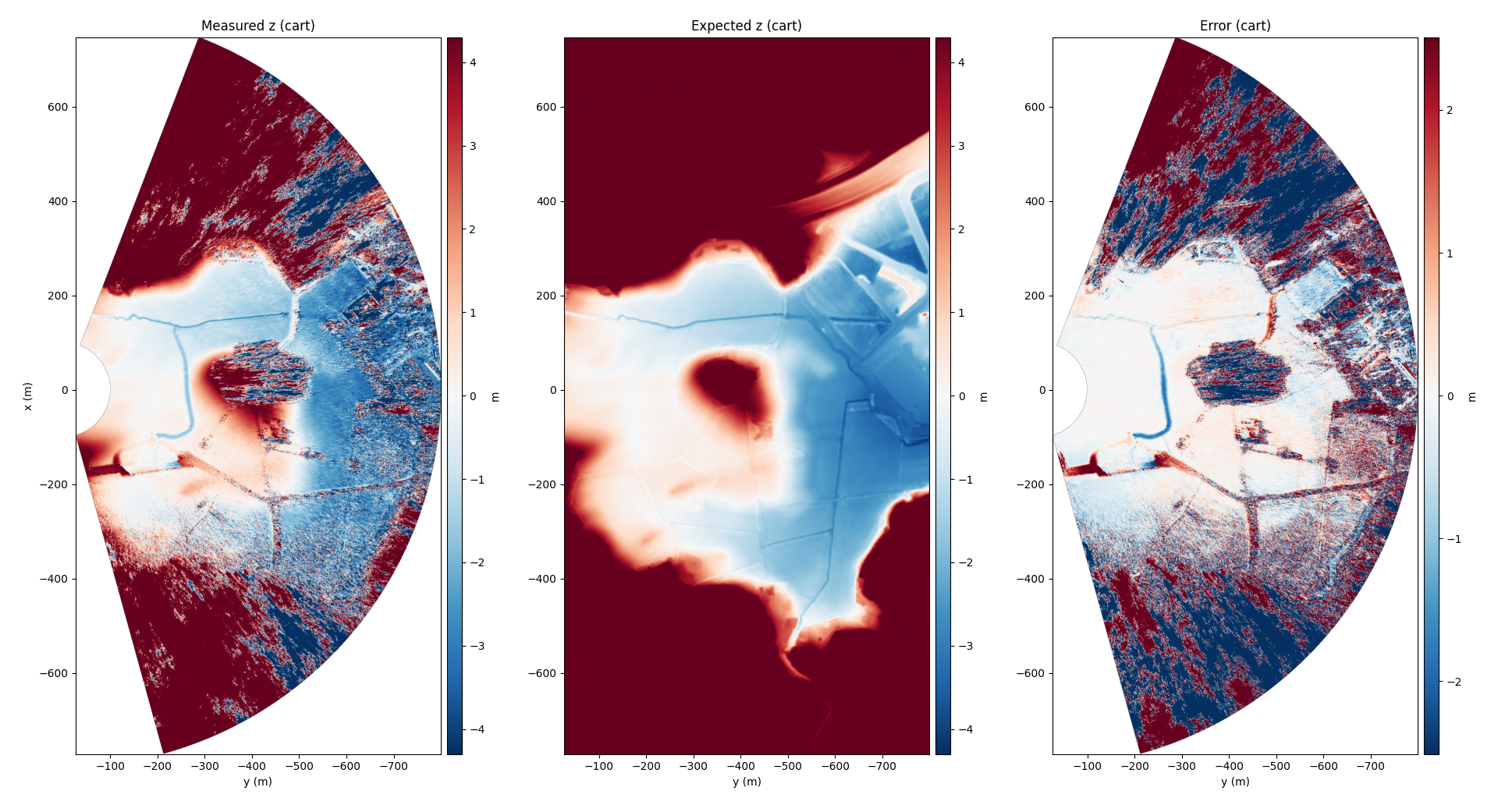
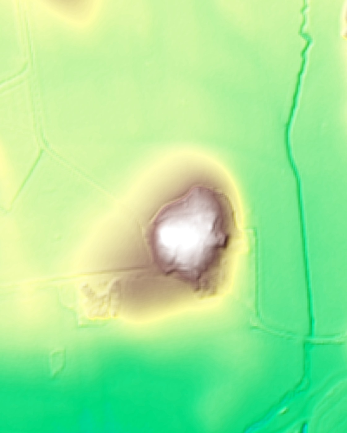
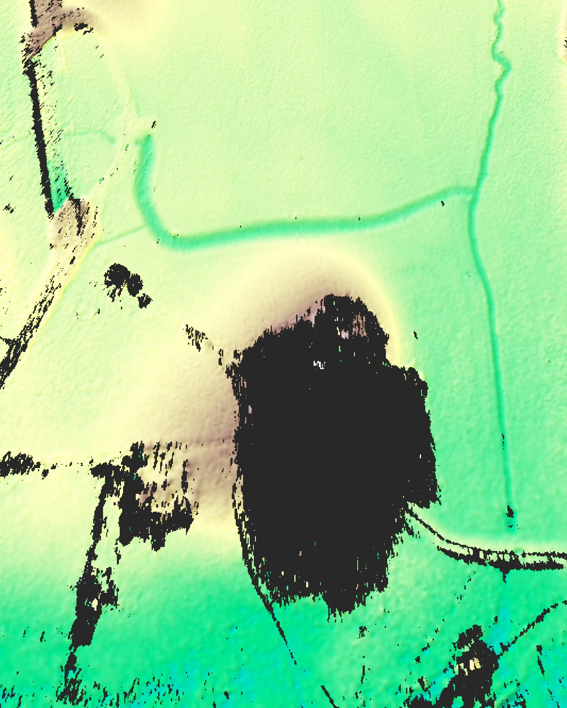 SAR DEMLidar DEM

Comparing the SAR and lidar DEMs, the SAR DEM has big holes in the decorrelated regions where phase measurement is too noisy to be used. However, the comparison is not completely fair since the SAR DEM was taken from a low altitude at a very shallow grazing angle, while the lidar is from an airplane high up looking nearly straight down. The SAR DEM that was generated referenced to the take-off height was shifted to N2000 height that the lidar reference uses for equal comparison.
The SAR interferogram's noise increases at far distances and in this plot a range-dependent filter was applied to keep the noise similar over the whole image at the expense of poorer resolution at far ranges. The RMS height difference is 0.4 m and the median absolute error is 0.11 m including the differing areas.
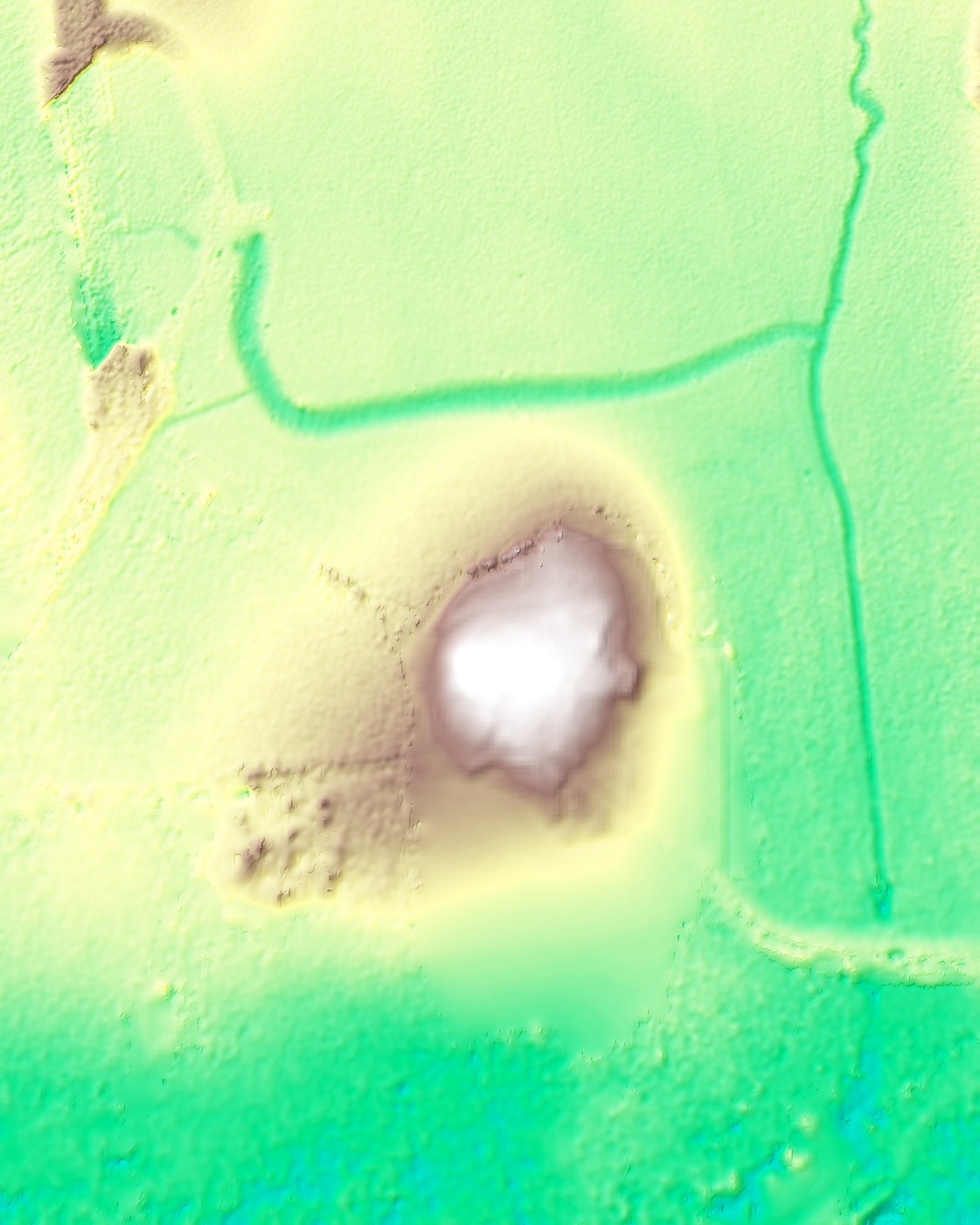 SAR DEM, filledLidar DEM
The missing pieces of the SAR DEM can be filled from the reference DEM giving this completed updated DEM over the area. Coherence is used for smoothing near the gaps. The maps agree well over the region and filling doesn't cause any seams. The bridge region is incorrect though since both SAR DEM unwrapping and the reference DEM are incorrect there.
Second mission
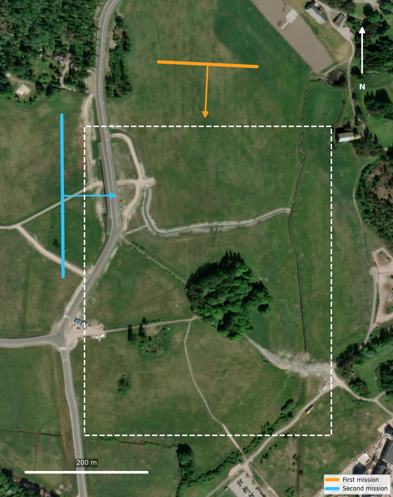
The mission tracks on a satellite map.
A second mission was flown with a 90 degree rotated flight track over the same area directly after the first mission with just a few minutes in between them. The dashed box shows the outline of the detail area before. The arrow shows the mean pointing of the antenna during the measurement. Both missions have a 1 m vertical baseline.
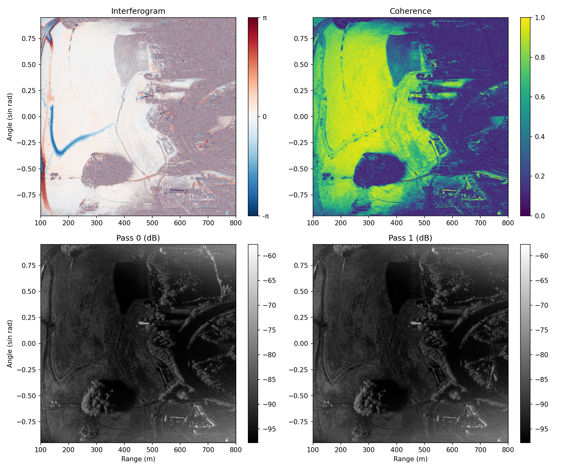
Interferogram on DEM, coherence, and amplitude images.
The second measurement also has high coherence after autofocus and RME. The mean coherence over the image is 0.480 including decorrelated regions. The field has very high coherence.
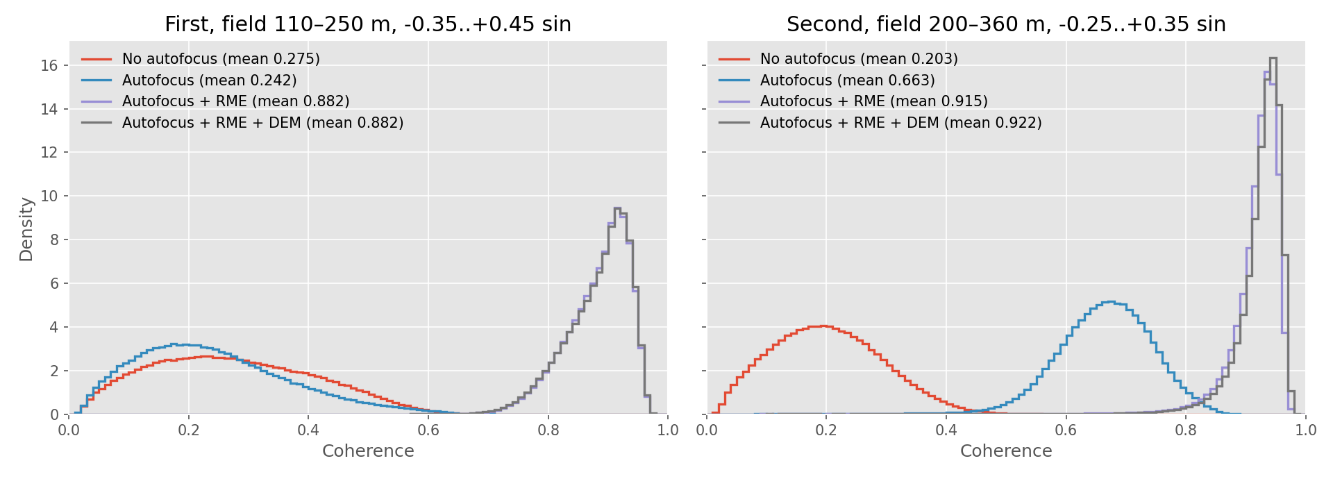
Coherence histogram.
Plotting the coherence histogram on both missions limited only to the field area (different on each image) shows how much RME helps. Without autofocus or RME both measurements are very poorly correlated between the passes with almost zero coherence. With autofocus and RME the coherence is very close to 1. The first mission has the field closer to the radar and I think the different look angle causes the scene to reflect slightly differently lowering the coherence. I tried common-band filtering too but it increases coherence only by 0.008 on average.
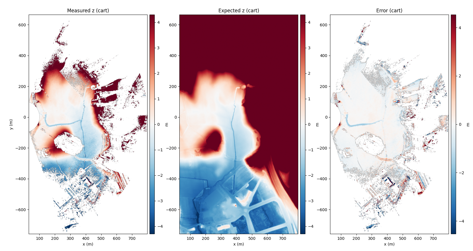
DEM from the other flight.
The DEM generated from the other flight with a rotated track also matches the reference well. It's also consistent with the earlier radar capture showing the same differences to the reference lidar elevation map. In this mission the solved baseline error is smaller, only (4.7, 0.2, -2.1) mm.
SAR data viewer
This widget shows both SAR measurements and the reference data over the same 400 x 500 m area.

The second mission track is not as well positioned for this area as the first mission. At the bottom left, the azimuth angle is almost 90 degrees for the second mission image and the antenna gain is very low at that extreme angle leading to low signal to noise ratio. The antenna radiation pattern from simulation that is used to normalize the image also doesn't quite agree with the real antenna especially at extreme angles which causes polarimetric errors at near ranges. Some of the polarimetric differences can be caused by the look angle as the polarimetric return can change depending on the angle. Both the vertical look angle and the azimuth angle of the target can cause differences between the images. At the top right edge of the image both of the missions have good illumination and the SAR images look similar. The second mission with the longer track has better resolution at that location, which is why it looks sharper there.
In this comparison the layover in SAR can be observed clearly. An elevated object will appear to be falling towards the radar due to the radar actually measuring the distance to the object. The top of a tall object is closer to the drone than the base near the ground causing it to appear closer to the radar in the image. With DEM used in image formation, the elevation difference of the ground is already compensated and it won't cause layover. The layover is very severe on the bridge and the forest regions, with a large difference between the SAR images. The garden at the bottom right also has some layover from the trees there.
The measured phase from elevation difference depends on both the baseline and the distance to the target. Since both are different, the phases don't cancel out between the missions. The SAR DEM should represent the same area and it should be comparable, but there are some unwrapping errors near the bridge and at farther ranges the noise in the two images scales differently. On average though, they do agree over the area.
The 1 m vertical baseline used here is fine for the close ranges, but far ranges could use a longer baseline to increase the elevation-to-phase sensitivity which would decrease noise in the generated DEM.
Summary
The radar drone is able to generate very high quality SAR images and high coherence interferograms between multiple measurements. A new residual motion estimation algorithm for interferometric SAR was described that makes this possible. The whole system is built by me on my own time with a total hardware cost of only about 1000 EUR including both the radar and the drone, a small fraction of what similar commercial interferometric SAR systems cost. The hardware is not for sale, but the SAR processing code is available in the torchbp Github repository licensed under the MIT license.